7 Components, Communities and Cliques
The study of group dynamics would be pretty ineffective if we were not able to identify and study important subgroups. Networks of people are often made up of subsets that interact more intensely among each other than they do with the rest of the network, and it is often very important in research and analysis to identify or approximate these subsets as best as possible so that they can be studied more closely. In complex networks, this is not an easy task. Most of the computational methods we have available to us for finding densely connected subsets of vertices (usually called communities) are iterative approximations which make use of heuristics62 and are rarely 100% accurate63. However, in the study of networks in the organizational sciences, we do not need high levels of precision to be able to draw valuable insights, and therefore these modern approximation techniques are very powerful tools for us to have at our disposal.
In the work we have done thus far in the book, we have already been exposed to subgraphs—we have used induced vertex subgraphs containing a specified set of vertices and all edges between them. However, in these situations we were able to specify the precise subset of vertices that we were interested in. In this chapter we will look at methods to identify or ‘detect’ subsets of vertices based on certain properties of the induced subgraphs of those vertices. We will start with simpler problems such as identifying subsets of vertices which are completely disconnected from others, and then we will proceed to look at graph partitioning and the identification of cliques and communities of vertices which, though not disconnected from other parts of the graph, have higher levels of density between each other than with the rest of the network.
7.1 Theory of components, partitions and clusters
7.1.1 Connected components of graphs
We learned earlier that a graph \(G\) is connected if a path exists between any pair of vertices \(u\) and \(v\) in \(G\). If \(G\) is a directed graph, we say \(G\) is weakly connected if it would be connected when viewed as an undirected graph. We say that \(G\) is strongly connected if a path exists from \(u\) to \(v\) for any pair of vertices \(u\) and \(v\) in \(G\). We say \(G\) is unilaterally connected if a path exists either from \(u\) and \(v\) or from \(v\) to \(u\) for any pair of vertices \(u\) and \(v\) in \(G\).
A connected component of a graph is a connected subset of vertices, none of which are connected to any other vertex in the graph. As an example, the undirected graph in Figure 7.1 consists of three connected components, each with three vertices. In the directed graph in Figure 7.2, one component is strongly connected (\(A \longrightarrow B \longrightarrow C \longrightarrow A\)), one is unilaterally connected (\(D \longrightarrow E \longrightarrow F\)) and the third is weakly connected (\(G \longrightarrow I \longleftarrow H\)).
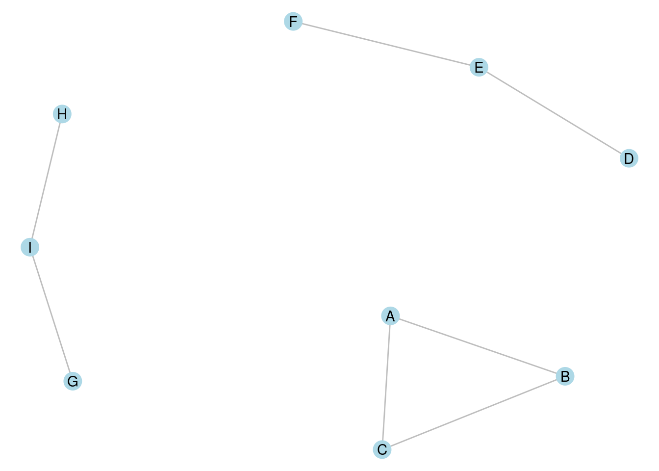
Figure 7.1: A graph with three connected components, each containing three vertices
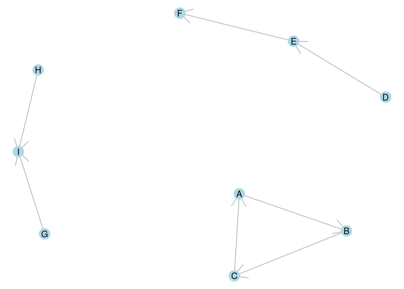
Figure 7.2: A directed graph with three connected components, one strongly connected, one weakly connected and one unilaterally connected
Connected components of disconnected graphs are important to identify because many of the measures we have learned so far break down for disconnected graphs. For example, the diameter of a disconnected graph is theoretically defined as infinite by mathematical convention, but this is not a useful practical measure. Usually when we want to know the diameter of a graph, we want to understand the largest finite distance between any two vertices, which translates to the diameter of the largest connected component in the graph. Therefore, most calculations of diameter in disconnected graphs require us to be able to identify the largest connected component.
It is not too difficult to think of an algorithm that can determine all the connected components of a graph. If you are interested in this, see the exercises at the end of this chapter.
Playing around: Go back and try to find some examples in earlier chapters of graphs that are disconnected, and calculate the diameter that is returned by the functions in R or Python packages. For example, you could try the Random Acts of Pizza graph from the exercises at the end of Chapter 3 or the graph of reported friendships from the schoolfriends data set at the end of the previous chapter. What do diameter functions return for these graphs?
7.1.2 Vertex partitioning
Often graphs will be connected, but we still want to divide the vertices up into mutually exclusive subgroups of interest. Such a division is called a partition of a graph. In a partition, all vertices must be in one and only one subgroup. Partitions are created through making cuts in a graph.
A cut in a graph \(G\) is a set of edges that divide the vertices of \(G\) into two disjoint subsets. The number of edges is known as the size of the cut. In Figure 7.3, edges e3, e4 and e5 divide the graph into two disjoint connected sets and represents a cut of size 3.
A minimum cut is a cut where no other cut exists in \(G\) with a smaller number of edges. In Figure 7.3, it should not be difficult to see that mimimum cuts have size 1 and can be achieved with either e1 or e2. In both cases, these minimum cuts divide the graph into a connected component and an isolate64.
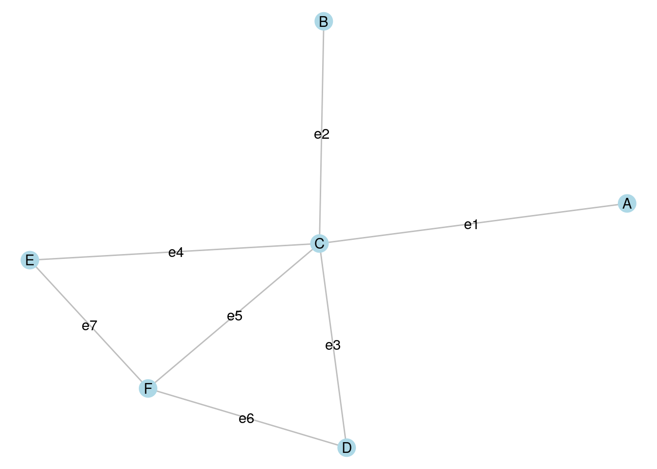
Figure 7.3: Cuts are defined by edges that split the vertices of a graph into disjoint subsets
A partition of a graph \(G\) is obtained through a series of cuts. For example, if we make a cut using e3, e5 and e7 in Figure 7.3, we split the graph into two disjoint connected graphs. If we then make a further cut using e1, we split the graph into three disjoint sets: two disjoint connected sets and an isolate.
In directed graphs, cuts can be defined according to the direction of edges, and in weighted graphs, minimum cuts can be determined through the weights of edges. The most popular algorithm for determining the minimum cut of a graph is the Stoer-Wagner algorithm (Stoer & Wagner (1997)).
7.1.3 Vertex clustering and community detection
Vertex clustering refers to the process of partitioning a graph in order to satisfy a certain objective. Most commonly in organizational network analysis, that objective is to achieve a high edge density between the vertices inside a cluster, and a low edge density between vertices that are in different clusters. Such highly connected clusters are usually referred to as communities and the process of determining optimal communities in a graph is known as community detection or community discovery65. Community detection is an unsupervised process. When we perform community detection on a graph, we do not know in advance how many communities we seek to find or the size of those communities.
The most commonly used (and fastest) community detection algorithm is the Louvain algorithm. The Louvain algorithm partitions a graph into subsets of vertices by trying to maximize the modularity of the graph. Modularity measures how dense the connections are within subsets of vertices in a graph by comparing the density to that which would be expected from a random graph. In an unweighted and undirected graph, modularity takes a value between \(-0.5\) and \(+1\). Any value above zero means that the vertices inside the subgroups are more densely connected than would be expected by chance. The higher the modularity of a graph, the more connected the vertices are inside the subgroups compared to between the subgroups, and therefore the more certain we can be that the subgroups represent genuine communities of more intense connection. The approximate steps of the Louvain algorithm are as follows:
- The algorithm starts its first phase with each vertex in its own community.
- Vertices are moved into other communities, and modularity is calculated.
- When the algorithm reaches a point where further vertex moves do not increase modularity, it finishes its first phase.
- In its second phase, the communities resulting from the first phase are aggregated to form a simpler pseudograph where each vertex represents a community, where loop edges on a vertex are weighted by the total number of edges inside that community, and where edges between vertices are weighted by the total number of edges between those communities66. In this heuristic step, vertices are moved in this simpler graph with the aim of improving modularity. That is, communities may be combined if modularity is improved.
- The first and second phases are repeated until modularity cannot be further improved.
A more recently developed community detection algorithm which improves on the Louvain algorithm is the Leiden algorithm. The Leiden algorithm operates similarly to Louvain, but has an additional refinement process at the end of the first phase which helps increase the options for improved modularity in the second phase. The Leiden algorithm will always achieve results as good as the Louvain algorithm, and in many cases may detect communities which are better connected than those detected by Louvain.
Both the Louvain and Leiden algorithms are good options for performing community detection in an organizational context. However, there are numerous other options, many of which are available in common data science packages. For example, the Girvan-Newman algorithm operates in a very different way by starting with an entire graph and progressively removing important edges to potentially reveal high modularity subgroups. For a more detailed reference on the Louvain and Leiden algorithms, see Traag et al. (2019) and for more general insight into a broader range of community detection algorithms, see Yang et al. (2016).
One important aspect of community detection which is often not understood is that community detection algorithms classify vertices into subgroups, but offer no direct insight into the nature of those subgroups. Further analytic techniques need to be applied to help describe the subgroups in a meaningful way. For example, the subgroups could be compared to known ‘ground truth’ characteristics of the network (such as department in the workfrance graph or class in the schoolfriends graph). We will examine this using an example later in this chapter.
7.1.4 Cliques
A clique is a subset of vertices in an undirected graph whose induced subgraph is complete. That is, the induced subgraph has an edge density of 1. This is best understood as the most intense possible type of community in an undirected graph. A maximal clique is a clique which cannot be extended by adding another vertex. A largest clique is a clique with the greatest number of vertices of all cliques in the graph.
In Figure 7.3, the following are maximal cliques: \(B \longleftrightarrow C\), \(A \longleftrightarrow C\), \(C \longleftrightarrow E \longleftrightarrow F\) and \(C \longleftrightarrow D \longleftrightarrow F\) because no other vertex can be added to these cliques without creating an incomplete graph. \(C \longleftrightarrow E \longleftrightarrow F\) and \(C \longleftrightarrow D \longleftrightarrow F\) are largest cliques because there is no clique in the graph that has more than three vertices.
Finding a single maximal clique in an undirected graph is not a complex problem and can be done quickly using a standard search algorithm starting on an arbitrary vertex. However, finding maximal cliques of a specified size, or all maximal cliques, as well as finding largest cliques, are problems whose complexity increases with the size and density of a graph. Care should be taken in attempting these algorithms on very large graphs.
Thinking ahead: Go back to the graph of Zachary’s Karate Club in Chapter 3. Can you identify some maximal cliques? What do you think is the size of the largest clique? Thinking about this will give you a sense of how hard the largest clique problem might be on very large graphs. We will use this as an example later in the chapter.
7.2 Finding components, communities and cliques using R
7.2.1 Finding connected components of disconnected graphs
To illustrate the components() function in igraph we will load up the schoolfriends edgelist data set from an earlier chapter. We will use reported friendships, create a directed graph and visualize it as in Figure 7.4.
library(igraph)
library(ggraph)
library(dplyr)

# get schoolfriends edgelist
schoolfriends_edgelist <- read.csv(
  "https://ona-book.org/data/schoolfriends_edgelist.csv"
)

# just use reported friendships
schoolfriends_reported <- schoolfriends_edgelist |>
  dplyr::filter(type == "reported")

# create directed graph
schoolfriends_rp <- igraph::graph_from_data_frame(
  schoolfriends_reported
)

# visualize
set.seed(123)
ggraph(schoolfriends_rp) +
  geom_edge_link(color = "grey",
                 arrow = arrow(length = unit(0.2, "cm"))) +
  geom_node_point(size = 2, color = "blue") +
  theme_void()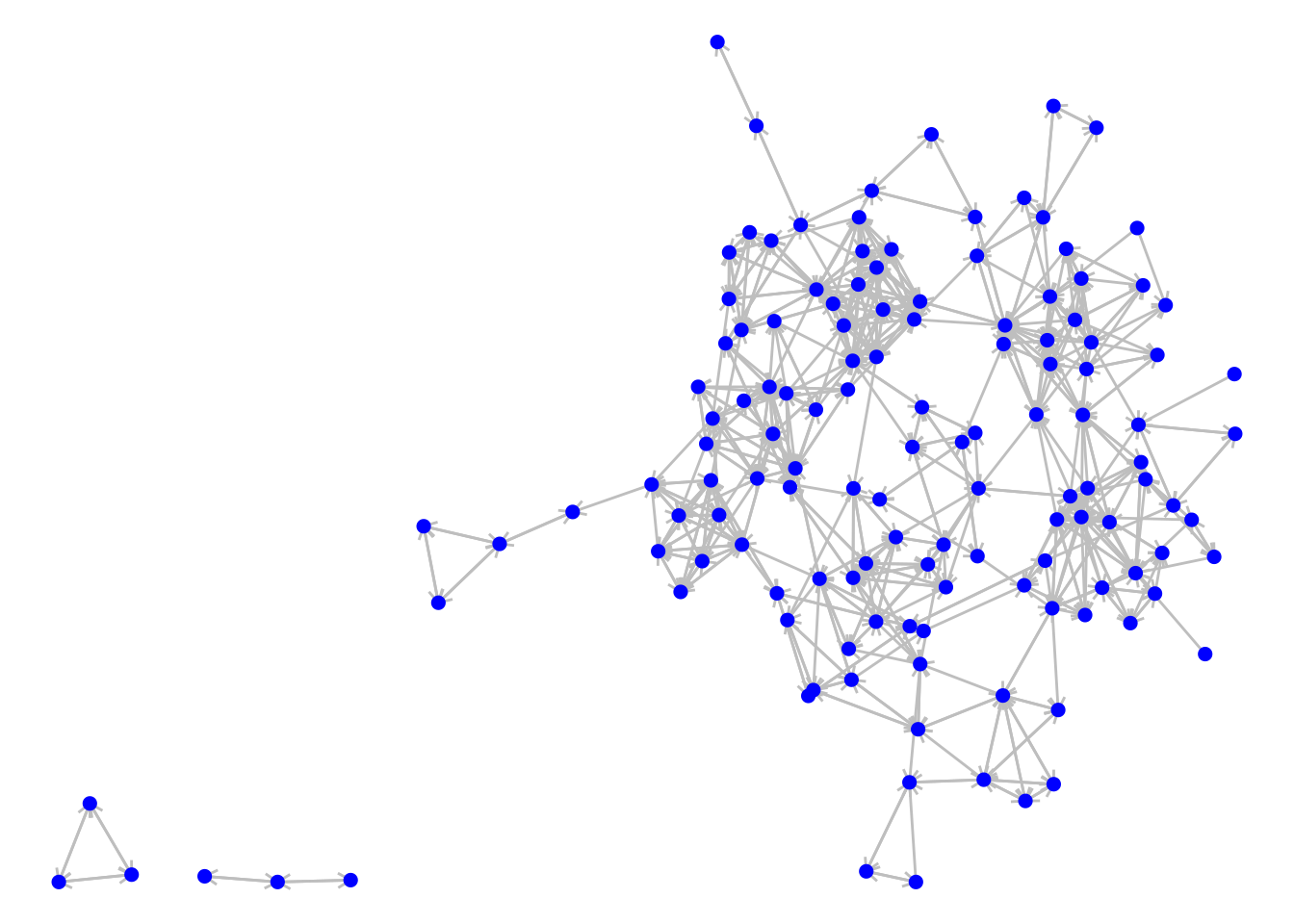
Figure 7.4: The directed graph of reported friendships from our French high school
We can see some connected components in this disconnected graph. We can use the components() function to classify the vertices into the connected components. This function generates a list containing the following vectors:
-
membership, which is a vector assigning each vertex to a numbered component -
csize, which returns the size of each component -
no, which is the number of connected components
Let’s verify the latter two:
# get weakly connected components (mode ignored if undirected)
schoolfriends_components <- igraph::components(schoolfriends_rp,
                                               mode = "weak")

# how many components?
schoolfriends_components$no
## [1] 3
# size of components
schoolfriends_components$csize
## [1] 128 3 3We can use the membership to assign a component property and then visualize with the vertices colored by component, as in Figure 7.5.
# assign component property
V(schoolfriends_rp)$component <- schoolfriends_components$membership

# visualize
ggraph(schoolfriends_rp) +
  geom_edge_link(color = "grey",
                 arrow = arrow(length = unit(0.2, "cm"))) +
  geom_node_point(size = 2, aes(color = as.factor(component))) +
  labs(color = "Component") +
  theme_void()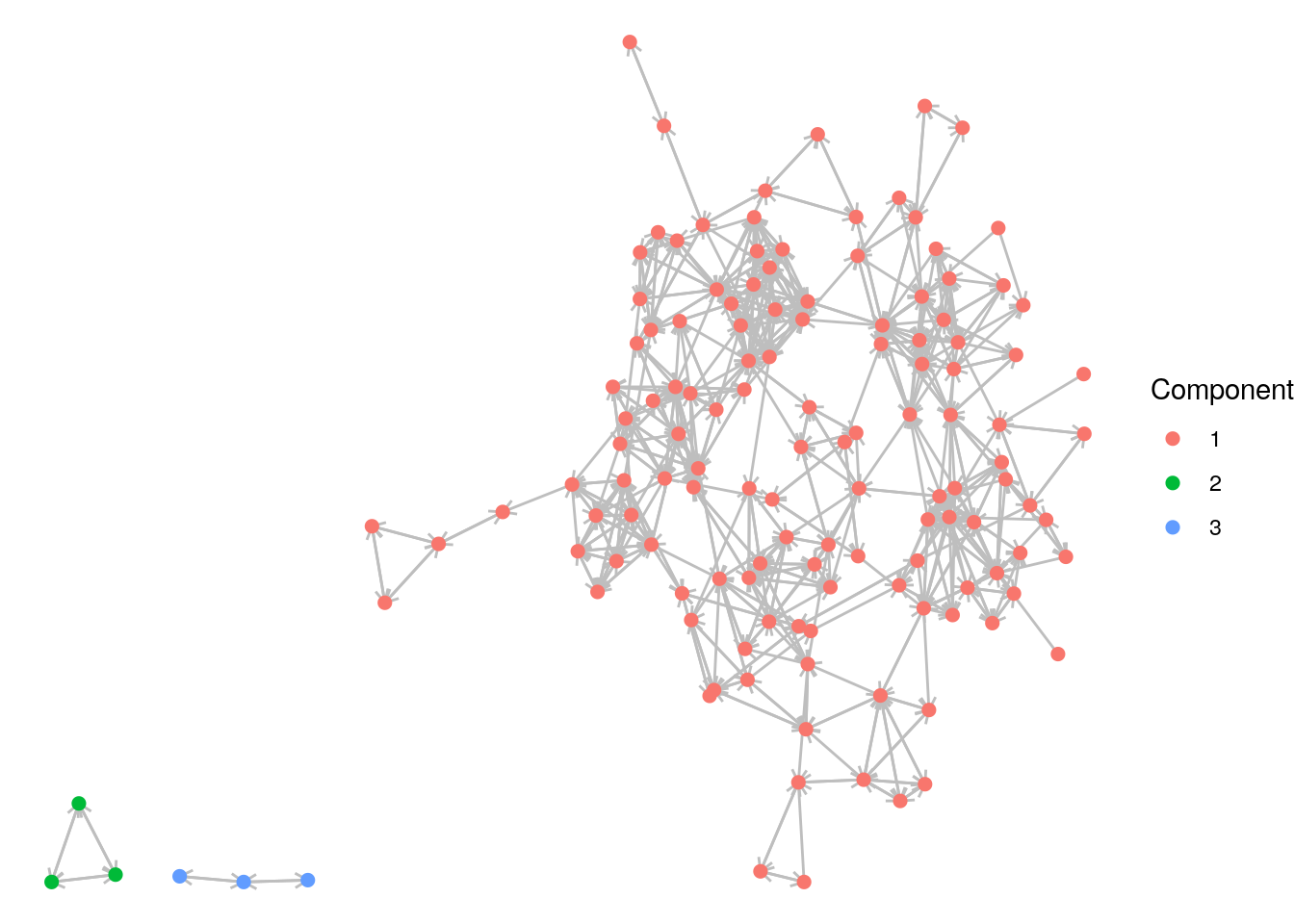
Figure 7.5: The reported schoolfriends graph color coded by its (weakly) connected components
Playing around: Weakly connected components of a directed graph are easier to spot with the naked eye compared to strongly connected components. Why? Remind yourself of the definition of weakly connected components from earlier in this chapter. Try to repeat this analysis to visualize all strongly connected components in the reported schoolfriends graph and see the difference.
7.2.2 Partitioning and community detection in R
For the next few examples, we will return to Zachary’s Karate Club network from Chapter 3. Let’s load up and visualize that undirected graph and mark the known leading actors Mr Hi and John A with larger vertices, as in Figure 7.6.
# get karate edgelist and create undirected graph
karate_edges <- read.csv("https://ona-book.org/data/karate.csv")
karate <- igraph::graph_from_data_frame(karate_edges, directed = FALSE)

# color John A and Mr Hi differently
V(karate)$leader <- ifelse(
  V(karate)$name %in% c("Mr Hi", "John A"), 1, 0
)

# visualize
set.seed(123)
ggraph(karate, layout = "fr") +
  geom_edge_link(color =  "grey") +
  geom_node_point(aes(size = as.factor(leader)), color = "blue",
                  show.legend = FALSE) +
  theme_void()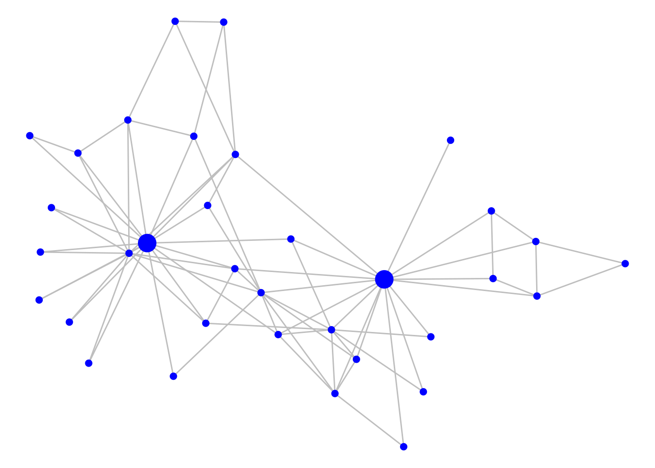
Figure 7.6: Zachary’s Karate Club graph with Mr Hi and John A indicated with larger vertices
Minimum cuts in graphs can be found using the min_cut() function in igraph. This will return the number of edges in the minimum cut, unless you use the value.only = FALSE argument, in which case it will return more information on the cut,
igraph::min_cut(karate, value.only = FALSE)## $value
## [1] 1
##
## $cut
## + 1/78 edge from 12c6c99 (vertex names):
## [1] Mr Hi--Actor 12
##
## $partition1
## + 1/34 vertex, named, from 12c6c99:
## [1] Actor 12
##
## $partition2
## + 33/34 vertices, named, from 12c6c99:
## [1] Mr Hi Actor 2 Actor 3 Actor 4 Actor 5 Actor 6 Actor 7 Actor 9 Actor 10 Actor 14 Actor 15 Actor 16
## [13] Actor 19 Actor 20 Actor 21 Actor 23 Actor 24 Actor 25 Actor 26 Actor 27 Actor 28 Actor 29 Actor 30 Actor 31
## [25] Actor 32 Actor 33 Actor 8 Actor 11 Actor 13 Actor 18 Actor 22 Actor 17 John AWe see that a minimum cut exists of size 1 between Mr Hi and Actor 12.
The Louvain community detection algorithm can be run using the cluster_louvain() function. weights can be added as an argument, or will be used by default if the graph has a weight edge attribute (set weight = NA to avoid this). This will produce a list of community groups. The best way to record the resulting community membership is to assign it as a vertex property using the membership() function.
# detect communities using Louvain
communities <- cluster_louvain(karate)

# assign as a vertex property
V(karate)$community <- membership(communities)
Before visualizing the communities, we can see how many they are and their size67:
sizes(communities)## Community sizes
## 1 2 3 4
## 11 6 11 6We have four detected communities of varying sizes. As before, we can color code to visualize these, as in Figure 7.7.
set.seed(123)
ggraph(karate, layout = "fr") +
  geom_edge_link(color =  "grey") +
  geom_node_point(aes(size = as.factor(leader),
                      color = as.factor(community)),
                  show.legend = FALSE) +
  theme_void()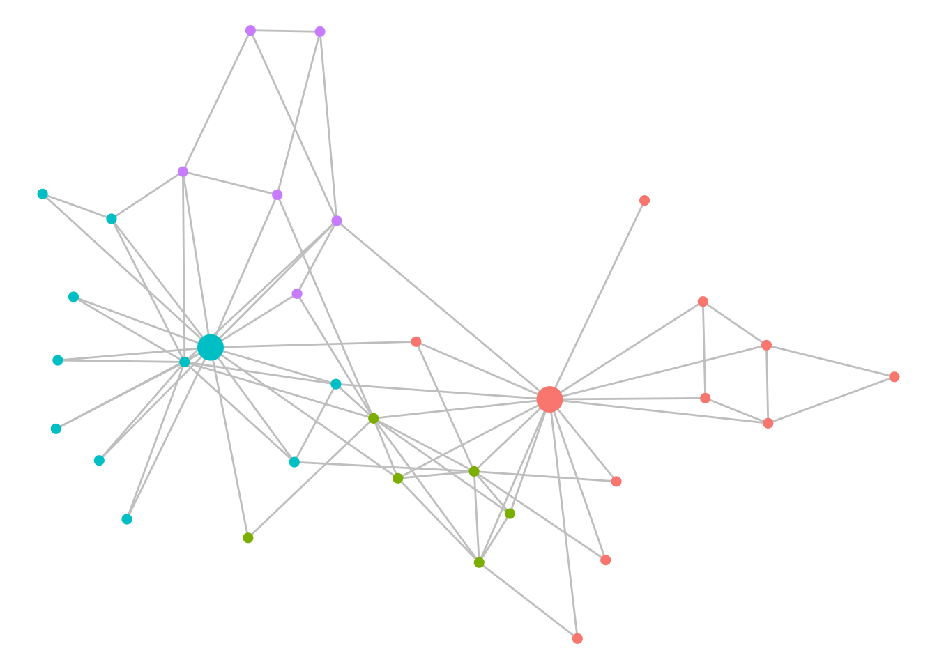
Figure 7.7: Communities of Zachary’s Karate Club as detected by the Louvain algorithm
Playing around:. Try playing around with some of the other community detection methods available in igraph using the karate example. How different are the results? For example, try cluster_edge_betweenness() (the Girvan-Newman algorithm) or cluster_infomap() or any other methods that begin with cluster.
7.2.3 Finding cliques in R
The cliques() and max_cliques() function in igraph identifies all cliques or maximal cliques, respectively, with a specified maximum or minimum size if desired. It is advisable to specify a size for cliques of interest because otherwise a long list might be returned, including many single node cliques.
max_cliques(karate, min = 5, max = 5)## [[1]]
## + 5/34 vertices, named, from 12c6c99:
## [1] Actor 2 Mr Hi Actor 4 Actor 3 Actor 14
##
## [[2]]
## + 5/34 vertices, named, from 12c6c99:
## [1] Actor 2 Mr Hi Actor 4 Actor 3 Actor 8The largest_cliques() function finds all largest cliques in a graph.
largest_cliques(karate)## [[1]]
## + 5/34 vertices, named, from 12c6c99:
## [1] Actor 2 Mr Hi Actor 4 Actor 3 Actor 14
##
## [[2]]
## + 5/34 vertices, named, from 12c6c99:
## [1] Actor 2 Mr Hi Actor 4 Actor 3 Actor 8We see that the maximal cliques of size 5 that we identified are also the largest cliques in the karate graph, and they have 4 out of 5 vertices in common. The function clique_num() returns the size of the largest clique.
clique_num(karate)## [1] 57.3 Finding components, communities and cliques using Python
7.3.1 Finding connected components using Python
For undirected graphs, the networkx function number_connected_components() returns the number of connected components in the graph, while the connected_components() function returns the vertices in each connected component.
For directed graphs, similar functions identify weakly and strongly connected components. Let’s use the reported friendships from the schoolfriends data set as an example.
import pandas as pd
import networkx as nx

# get schoolfriends edgelist
schoolfriends_edges = pd.read_csv(
  "https://ona-book.org/data/schoolfriends_edgelist.csv"
)

# use only reported friendships
schoolfriends_reported = schoolfriends_edges[
  schoolfriends_edges.type == "reported"
]

# create directed graph
schoolfriends_rp = nx.from_pandas_edgelist(
  schoolfriends_reported,
  source = "from",
  target = "to",
  create_using=nx.DiGraph
)

# number of weakly connected components
nx.number_weakly_connected_components(schoolfriends_rp)
## 3# create component subgraphs
components = nx.weakly_connected_components(schoolfriends_rp)
subgraphs = [schoolfriends_rp.subgraph(component).copy()
for component in components]
# size of subgraphs
[len(subgraph.nodes) for subgraph in subgraphs]## [128, 3, 3]## NodeView((366, 1485, 974))7.3.2 Partitioning and community detection using Python
networkx has numerous algorithmic functions for exploring edge cuts on graphs, including to find the minimum edge cut. You can consult the reference documentation68 to learn about the various functions available. Let’s use the karate data set to demonstrate how to find a minimum cut.
# get karate edgelist
karate_edges = pd.read_csv("https://ona-book.org/data/karate.csv")

# create undirected network
karate = nx.from_pandas_edgelist(karate_edges, source = "from",
target = "to")

# find minimum cut
nx.minimum_edge_cut(karate)
## {('Actor 12', 'Mr Hi')}## 1Various built-in community detection algorithms are available in the networkx.community module, such as the Girvan-Newman edge betweenness algorithm. This generates communities by progressively removing edges with the highest edge betweenness centrality. It returns an iterator object where the first element is the result of the first edge removal, and subsequent elements are the result of progressive edge removal.
# get communities based on girvan-newman and sort by no of communities
communities = sorted(
  nx.community.girvan_newman(karate),
  key = len
)

# view communities from first edge removal
pd.DataFrame(communities[0]).transpose()
## 0 1
## 0 Actor 22 Actor 16
## 1 Actor 11 Actor 15
## 2 Mr Hi Actor 29
## 3 Actor 17 Actor 27
## 4 Actor 2 Actor 10
## 5 Actor 7 John A
## 6 Actor 13 Actor 19
## 7 Actor 4 Actor 24
## 8 Actor 6 Actor 3
## 9 Actor 5 Actor 26
## 10 Actor 8 Actor 32
## 11 Actor 18 Actor 25
## 12 Actor 20 Actor 31
## 13 Actor 14 Actor 23
## 14 Actor 12 Actor 9
## 15 None Actor 30
## 16 None Actor 28
## 17 None Actor 21
## 18 None Actor 33We see that the first split leads to two communities, one around John A and the other around Mr Hi.
The cdlib package in Python contains a very wide range of community detection algorithms that work with the networkx package, including the Louvain and Leiden algorithms as well as many others. In this example, we create a Louvain partition of the karate graph using cdlib.
from cdlib import algorithms
import numpy as np
import matplotlib.cm as cm
import matplotlib.pyplot as plt

# get louvain partition which optimizes modularity
louvain_comms = algorithms.louvain(karate)
louvain_comms is a clustering object that has a lot of useful properties and methods. To see the communities, use the following:
##            0         1         2         3
## 0      Mr Hi   Actor 9  Actor 32   Actor 5
## 1    Actor 2  Actor 31  Actor 28   Actor 6
## 2    Actor 3  Actor 33  Actor 29   Actor 7
## 3    Actor 4    John A  Actor 24  Actor 11
## 4    Actor 8  Actor 15  Actor 26  Actor 17
## 5   Actor 12  Actor 16  Actor 25      None
## 6   Actor 13  Actor 19      None      None
## 7   Actor 14  Actor 21      None      None
## 8   Actor 18  Actor 23      None      None
## 9   Actor 20  Actor 30      None      None
## 10  Actor 22  Actor 27      None      None
## 11  Actor 10      None      None      None
We see four communities. The modularity of the resulting community structure can be calculated using the newman_girvan_modularity() method.
## FitnessResult(min=None, max=None, score=0.4188034188034188, std=None)To visualize the network community structure, we can create a color mapping against the communities, as in Figure 7.8.
import matplotlib.pyplot as plt
from matplotlib import cm
from matplotlib.colors import ListedColormap, LinearSegmentedColormap

# create dict with labels only for Mr Hi and John A
node = list(karate.nodes)
labels = [i if i == "Mr Hi" or i == "John A" else "" \
for i in karate.nodes]
nodelabels = dict(zip(node, labels))

# create and order community mappings
communities = louvain_comms.to_node_community_map()
communities = [communities[k].pop() for k in node]

# create color map
pastel2 = cm.get_cmap('Pastel2', max(communities) + 1)

# visualize
np.random.seed(123)
nx.draw_spring(karate, labels = nodelabels, cmap = pastel2,
node_color = communities, edge_color = "grey")
plt.show()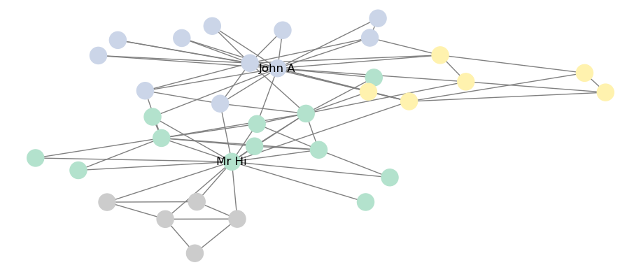
Figure 7.8: Best Louvain partition of Zachary’s Karate Club graph
Playing around: The options for community detection algorithms in the cdlib Python package are extensive. Consider playing around with some different algorithms. For example, you could try to visualize the community structure based on the Leiden algorithm. It’s also worth spending a little time exploring the technical documentation for the cdlib package69 to see the range of methods available.
7.3.3 Finding cliques in Python
All maximal cliques in a graph can be calculated using the find_cliques() function:
cliques = nx.find_cliques(karate)
maximal_cliques = sorted(cliques, key = len)

# get number of maximal cliques
len(maximal_cliques)
## 36## ['Mr Hi', 'Actor 2', 'Actor 4', 'Actor 3', 'Actor 14']Alternatively, there are functions that can calculate the number of cliques, the size of the largest clique, and can extract the graph of the largest clique.
## 36## 57.4 Examples of uses
In this section we will illustrate the implementation and interpretation of community detection algorithms using our Facebook schoolfriends example, and introducing a new example related to political tweets in the Ontario province of Canada.
7.4.1 Detecting communities and cliques among Facebook friends
Let’s reload our Facebook schoolfriends graph and remove any isolates so that we can investigate communities and cliques inside it.
# get schoolfriends data
schoolfriends_edgelist <- read.csv(
  "https://ona-book.org/data/schoolfriends_edgelist.csv"
)
schoolfriends_vertices <- read.csv(
  "https://ona-book.org/data/schoolfriends_vertices.csv"
)

# facebook friendships only
schoolfriends_facebook <- schoolfriends_edgelist |>
  dplyr::filter(type == "facebook")

# create undirected graph
schoolfriends_fb <- igraph::graph_from_data_frame(
  d = schoolfriends_facebook,
  vertices = schoolfriends_vertices,
  directed = FALSE
)

# remove isolates
isolates = which(degree(schoolfriends_fb) == 0)
schoolfriends_fb <- delete.vertices(schoolfriends_fb, isolates)
We now have a connected, undirected graph of 156 vertices, with class and gender as vertex properties. First, let’s detemine the largest clique in the graph.
(cliques <- igraph::largest_cliques(schoolfriends_fb))## [[1]]
## + 14/156 vertices, named, from 23c1636:
## [1] 1218 440 245 694 325 125 1423 841 376 466 624 1067 638 1237
##
## [[2]]
## + 14/156 vertices, named, from 23c1636:
## [1] 1218 440 245 694 325 125 1423 841 376 466 624 1067 638 797
##
## [[3]]
## + 14/156 vertices, named, from 23c1636:
## [1] 1218 440 245 694 325 125 1423 841 376 466 624 769 1237 638
##
## [[4]]
## + 14/156 vertices, named, from 23c1636:
## [1] 1218 440 245 694 325 125 1423 841 376 466 624 769 1237 564
##
## [[5]]
## + 14/156 vertices, named, from 23c1636:
## [1] 1218 440 245 694 325 125 1423 841 376 466 624 769 797 638
##
## [[6]]
## + 14/156 vertices, named, from 23c1636:
## [1] 1218 440 245 694 325 125 1423 841 376 466 525 769 797 638We see 6 cliques of 14 individuals, all of which have considerable overlap. We can take a look at the class and gender of one of these cliques.
# subgraph for clique 6
clique6 <- igraph::induced_subgraph(schoolfriends_fb,
                                    vids = cliques[[6]])

(data.frame(
  id = V(clique6)$name,
  class = V(clique6)$class,
  gender = V(clique6)$gender
))
## id class gender
## 1 466 MP*1 M
## 2 376 MP*1 M
## 3 638 MP*1 M
## 4 841 MP*1 M
## 5 1423 MP*2 M
## 6 1218 MP*2 M
## 7 769 PSI* M
## 8 797 PSI* F
## 9 440 PSI* F
## 10 125 PSI* F
## 11 325 PSI* M
## 12 694 MP F
## 13 245 MP F
## 14 525 MP FWe see that this clique is distributed over four classes and is mostly male. Let’s visualize where this clique sits in the full network, as in Figure 7.9.
# create clique property
V(schoolfriends_fb)$clique6 <- ifelse(
  V(schoolfriends_fb) %in% cliques[[6]], 1, 0
)

# visualize
set.seed(123)
ggraph(schoolfriends_fb, layout = "fr") +
  geom_edge_link(color = "grey", alpha = 0.7) +
  geom_node_point(size = 2, aes(color = as.factor(clique6)),
                  show.legend = FALSE) +
  theme_void()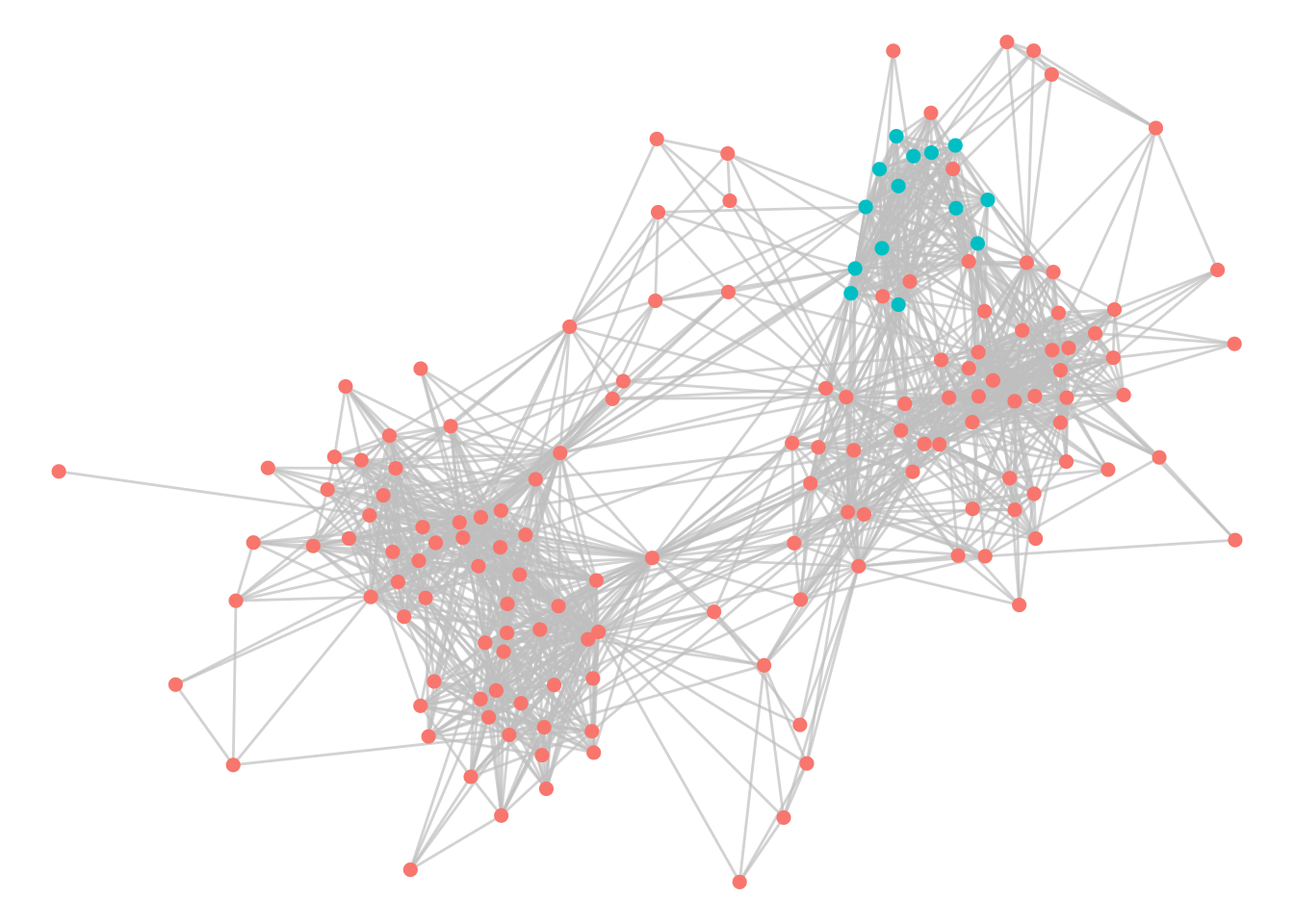
Figure 7.9: Facebook schoolfriends network with one of the largest cliques indicated
Now let’s use the Louvain algorithm to detect communities in our graph.
# get optimal louvain communities
communities <- igraph::cluster_louvain(schoolfriends_fb)

# assign community as a vertex property
V(schoolfriends_fb)$community <- membership(communities)

# how many communities?
length(unique(V(schoolfriends_fb)$community))
## [1] 6Six communities have been identified. Let’s compare the modularity of this community structure to the known ground truth communities of class and gender.
# modularity of louvain
modularity(schoolfriends_fb, V(schoolfriends_fb)$community)
## [1] 0.5290014
# modularity of class structure
modularity(schoolfriends_fb,
           as.integer(as.factor(V(schoolfriends_fb)$class)))
## [1] 0.317128
# modularity of gender structure
modularity(schoolfriends_fb,
           as.integer(as.factor(V(schoolfriends_fb)$gender)))
## [1] 0.06504432This community structure is certainly a better indicator of connected Facebook subgroups than gender or class. We can visualize the class structure side-by-side with the Louvain community structure to try to interpret it, as in Figure 7.10.
# use patchwork package for combining plots easily
library(patchwork)

# visualize louvain communities
set.seed(123)
g1 <- ggraph(schoolfriends_fb, layout = "fr") +
  geom_edge_link(color = "grey", alpha = 0.7) +
  geom_node_point(size = 2, aes(color = as.factor(community)),
                  show.legend = FALSE) +
  theme_void()

# visualize ground truth class communities
set.seed(123)
g2 <- ggraph(schoolfriends_fb, layout = "fr") +
  geom_edge_link(color = "grey", alpha = 0.7) +
  geom_node_point(size = 2, aes(color = class),
                  show.legend = FALSE) +
  theme_void()

# display side by side
g1 + g2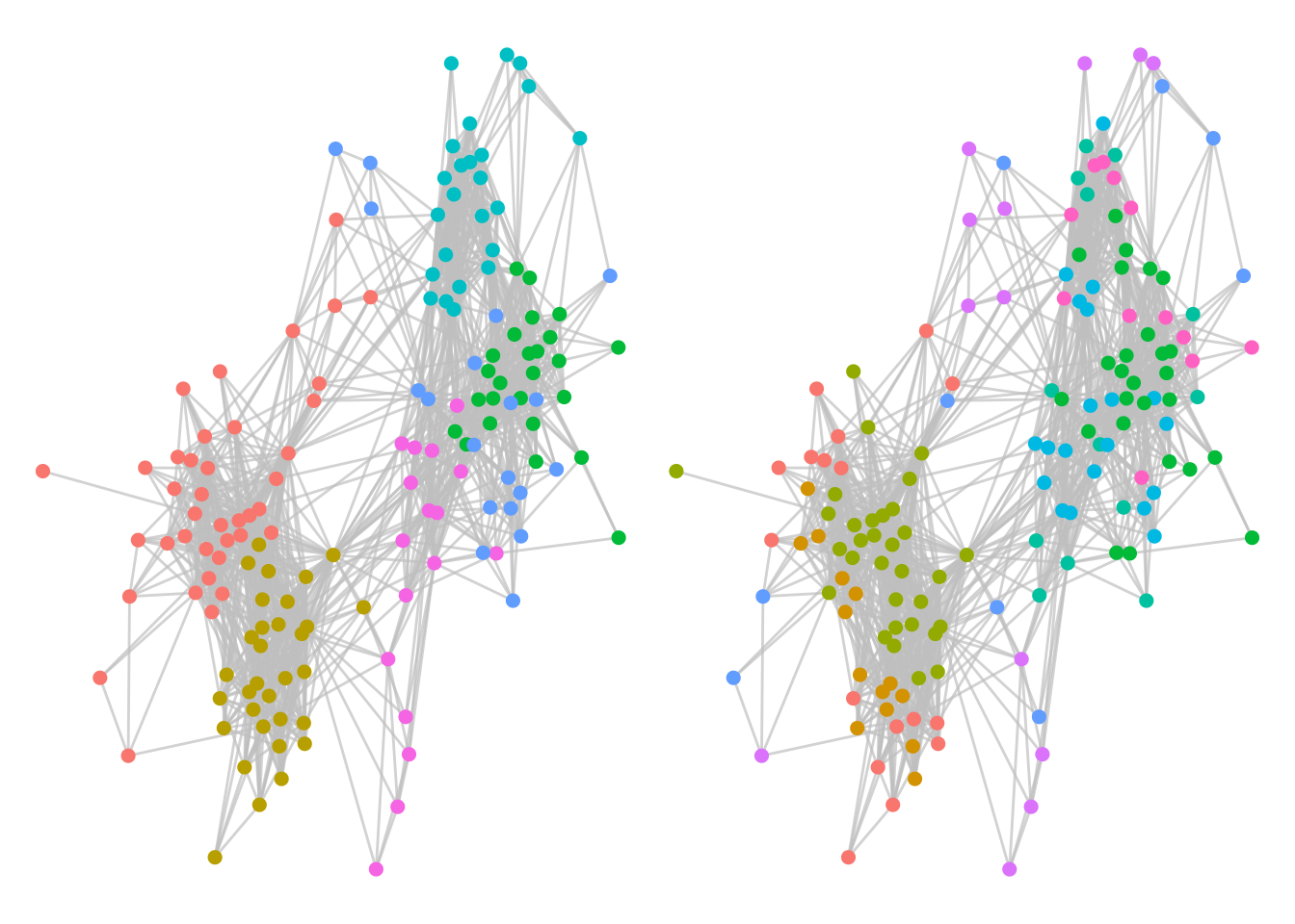
Figure 7.10: Optimal Louvain communities in the Facebook schoolfriends graph (left) versus ground truth class communities (right)
Visually, we can see that the Louvain community structure is a much better representation of dense friendship groups compared to the ground truth class structure, indicating that Facebook friendships tend to span across those class structures. We can also see that one of the Louvain communities contains the clique we identified earlier.
7.4.2 Detecting politically aligned communities on Twitter
The ontariopol_edgelist and ontariopol_vertices data sets represent tweeting activity between Ontario province politicians in Canada as captured in September 2021 and spanning several prior years of activity. Although the Twitter graph is a directed graph, we will set this network up as undirected, with two politicians connected if there has been an interaction between them by means of one mentioning the other in a tweet or one replying to a tweet from the other. The weight property represents the number of interactions and is therefore a measure of the connection strength.
# get edgelist and vertex data
ontariopol_edges <- read.csv(
  "https://ona-book.org/data/ontariopol_edgelist.csv"
)
ontariopol_vertices <- read.csv(
  "https://ona-book.org/data/ontariopol_vertices.csv"
)

# create undirected graph
(ontariopol <- igraph::graph_from_data_frame(
  d = ontariopol_edges,
  vertices = ontariopol_vertices,
  directed = FALSE
))
## IGRAPH 9bde201 UNW- 108 6095 --
## + attr: name (v/c), screen_name (v/c), party (v/c), weight (e/n)
## + edges from 9bde201 (vertex names):
## [1] Deepak Anand--Doug Ford Deepak Anand--Victor Fedeli Deepak Anand--Deepak Anand
## [4] Deepak Anand--Monte McNaughton Deepak Anand--Christine Elliott Deepak Anand--Stephen Lecce
## [7] Deepak Anand--Rod Phillips Deepak Anand--Lisa MacLeod Deepak Anand--Michael Tibollo
## [10] Deepak Anand--Peter Bethlenfalvy Deepak Anand--Raymond Sung Joon Cho Deepak Anand--Rudy Cuzzetto
## [13] Deepak Anand--Caroline Mulroney Deepak Anand--Sheref Sabawy Deepak Anand--Nina Tangri
## [16] Deepak Anand--Jill Dunlop Deepak Anand--Todd Smith Deepak Anand--Kinga Surma
## [19] Deepak Anand--Lisa Thompson Deepak Anand--Kaleed Rasheed Deepak Anand--Steve Clark
## [22] Deepak Anand--Ernie Hardeman Deepak Anand--Natalia Kusendova
## + ... omitted several edgesWe have an undirected, weighted graph, with screen_name and party vertex properties. First, we check if our graph is connected:
is.connected(ontariopol)## [1] TRUENow we use the Louvain algorithm to detect an optimal community structure in our graph. Since the graph has a weight property, our modularity calculations will include edge weight.
# find optimal communities
communities <- igraph::cluster_louvain(ontariopol)

# assign as vertex properties
V(ontariopol)$community <- membership(communities)

# how many communities
length(unique(V(ontariopol)$community))
## [1] 5We see six commmunities. Let’s compare the modularity of this community structure to the ground truth political party structure.
# louvain modularity
modularity(ontariopol,
           membership = V(ontariopol)$community,
           weights = E(ontariopol)$weight)
## [1] 0.3882044
# political party modularity
modularity(ontariopol,
           membership = as.integer(as.factor(V(ontariopol)$party)),
           weights = E(ontariopol)$weight)
## [1] 0.382394We see very similar modularity. Let’s visualize the Louvain community and party structure side-by-side, as in Figure 7.11.
# visualize louvain communities
set.seed(123)
g1 <- ggraph(ontariopol, layout = "fr") +
  geom_edge_link(color = "grey", alpha = 0.7) +
  geom_node_point(size = 2, aes(color = as.factor(community)),
                  show.legend = FALSE) +
  theme_void()

# visualize ground truth political party communities
set.seed(123)
g2 <- ggraph(ontariopol, layout = "fr") +
  geom_edge_link(color = "grey", alpha = 0.7) +
  geom_node_point(size = 2, aes(color = party),
                  show.legend = FALSE) +
  theme_void()

# display side by side
g1 + g2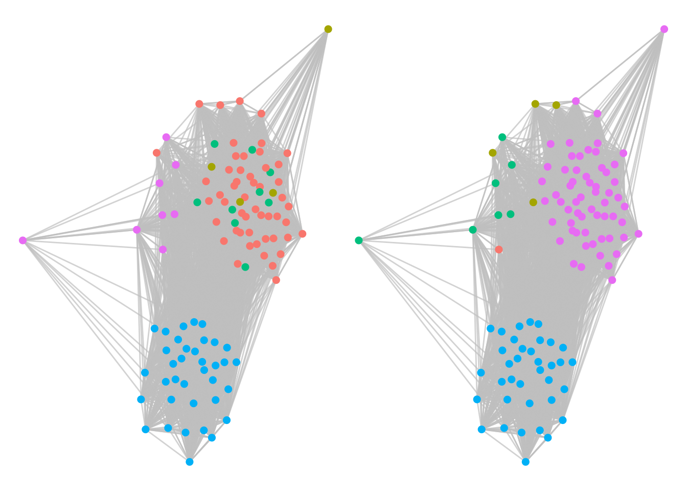
Figure 7.11: Twitter interaction of Ontario politicians segmented by their Louvain communities (left) and their ground truth political parties (right). Louvain does a good job of identifying political alignment.
We see very similar community structures, indicating that the Louvain algorithm has done a good job of identifying political party alignment from the tweet activity of the politicians. Using similar methods to our Facebook schoolfriends example in Section 7.4.1, we can also identify large cliques within the political parties, as in Figure 7.12.
# get largest cliques
cliques <- igraph::largest_cliques(ontariopol)

# there are 24 cliques of size 48 - choose one and visualize
# create clique property
V(ontariopol)$clique24 <- ifelse(
  V(ontariopol) %in% cliques[[24]], 1, 0
)

# visualize clique
set.seed(123)
g1 <- ggraph(ontariopol, layout = "fr") +
  geom_edge_link(color = "grey", alpha = 0.7) +
  geom_node_point(size = 2, aes(color = as.factor(clique24)),
                  show.legend = FALSE) +
  theme_void()

# visualize ground truth political parties
set.seed(123)
g2 <- ggraph(ontariopol, layout = "fr") +
  geom_edge_link(color = "grey", alpha = 0.5) +
  geom_node_point(size = 2, aes(color = party)) +
  labs(color = "Party (Right hand graph)") +
  theme_void()

g1 + g2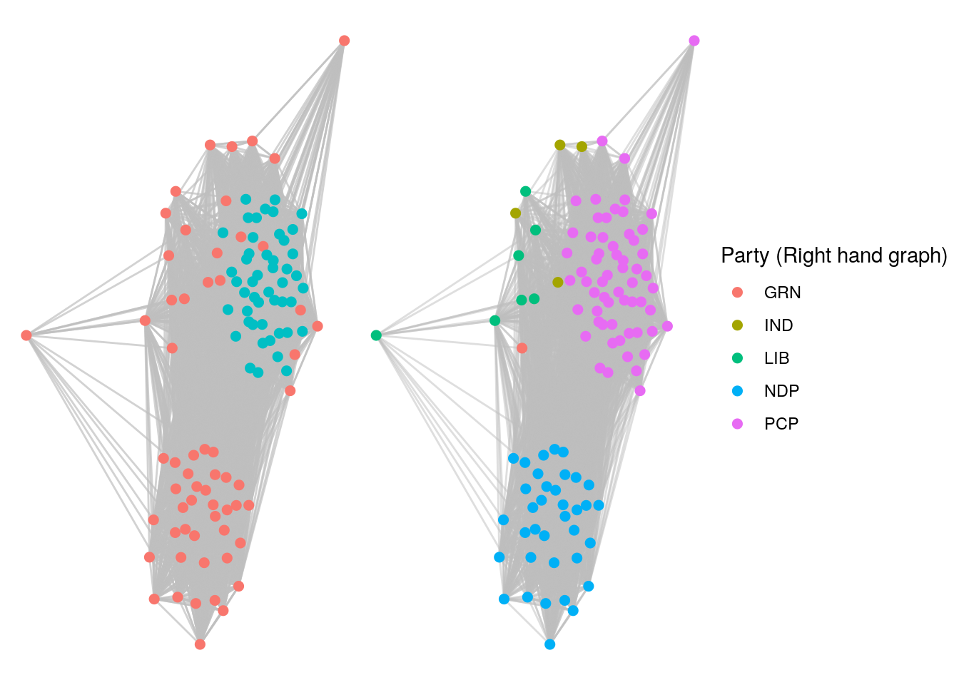
Figure 7.12: Large Twitter clique of 48 politicians (left). Comparison with party membership (right) reveals this to be a PCP clique.
Playing around: In both of the examples in this section, consider extending the work to identify key important or influential nodes within communities using your learning from Chapter 6. Remember that the Twitter graph is a directed graph and this may impact calculations of centrality, so consider moving back to a directed graph for these calculations. Also, try investigating what happens when you seek optimal unweighted Louvain communities in the ontariopol graph.
7.5 Learning exercises
7.5.1 Discussion questions
- What does it mean when an undirected graph is described as a connected graph? Provide similar definitions for a weakly and strongly connected directed graph.
- By starting with a random vertex, design a set of algorithmic steps that would determine all connected components of an undirected graph.
- What is a vertex partition of a graph? Describe how a partition arises from a series of edge cuts in a graph.
- What is meant by a vertex clustering of a graph?
- What is meant by a community of vertices? What objective are we usually trying to achieve when we detect communities in a graph?
- Describe your understanding of the term ‘modularity’ as it relates to community detection in graphs.
- Name a common community detection algorithm and describe how it works.
- What do we mean by the term ‘unsupervised’ when we describe a community detection process?
- What is meant by the term ‘clique’ in an undirected graph?
- What is a maximal clique and a largest clique in a graph? Are maximal cliques always largest cliques? Why or why not?
7.5.2 Data exercises
For Exercises 1-3, load the wikivote edgelist from the onadata package or download it from the internet70. Recall that this data set represents votes from Wikipedia members to other Wikipedia members to nominate the to member to administrator status. Create a directed graph from this data set. Be careful with trying to visualize this graph, as it is large.
- Determine how many weakly connected components there are in this graph. How large is the largest component?
- Determine how many strongly connected components there are in this graph. How large is the largest component?
- Describe how you would explain and interpret the difference between your results for Questions 1 and 2.
For Exercises 4-10, load the email_edgelist and email_vertices data sets from the onadata package or download them from the internet71. This data set represents a network of emails sent between members of a large research institution. The department of each member is included in the vertex data set. Create an undirected graph from this data72.
- Determine the connected components of this network and reduce the network to its largest connected component.
- Use the Louvain algorithm to determine a vertex partition/community structure with optimal modularity in this network.
- Compare the modularity of the Louvain community structure with that of the ground truth department structure.
- Visualize the graph color-coded by the Louvain community, and then visualize the graph separately color-coded by the ground truth department. Compare the visualizations. Can you describe any of the Louvain communities in terms of departments?
- Create a dataframe containing the community and department for each vertex. Manipulate this dataframe to show the percentage of individuals from each department in each community. Try to visualize this using a heatmap or other style of visualization and try to use this to describe the communities in terms of departments.
- Find the largest clique size in the graph. How many such largest cliques are there? What do you think a clique represents in this context?
- Try to visualize the members of these cliques in the context of the entire graph. What can you conclude?
Extension: These questions require the use of the Leiden community detection algorithm, which you may recall from earlier in this chapter is guaranteed to find a partition which at least matches the modularity of a Louvain partition, and can often improve it. If you are a Python programmer, the Leiden algorithm is easily used from the cdlib package. If you are an R programmer, you will need to use the leiden package, which uses a Python implementation of the algorithm inside R. You may need to be familiar with the reticulate package73 to ensure that an appropriate Python environment is available inside your R session.
- Use the Leiden community detection algorithm to find a vertex partition with optimal modularity. How many communities does the Leiden algorithm detect?
- Compare the Leiden partition modularity to the Louvain partition modularity.
- Try to use visualization or data exploration methods to determine the main differences between the Leiden and Louvain partitions.