5 Paths and Distance

Over the course of the earlier chapters, as we learned how to transform data into graph-friendly structures and how to create and visualize graphs, we started to see some concepts emerge informally which we will now start to formally describe and support by means of some mathematical definition and measurement. For example, we have seen that vertices can be connected directly or indirectly to other vertices by means of a single edge or a series of edges. We have observed visually that there can be greater ‘distance’ between some vertices in graphs compared to others, and in some cases it is simply not possible to get from one vertex to another along any edges in a graph.

The process of moving from vertex to vertex along edges in a graph is known as graph traversal. Graph traversal is an extremely important topic that underlies any sort of graph search algorithm. Graph search algorithms, in turn, are foundational in determining the optimal or shortest paths between pairs of vertices, or the set of shortest paths from a given vertex to all other vertices. Shortest paths are themselves important in the definition of distance and diameter in networks. Distance and diameter are useful and intuitive measurements that are frequently used in understanding ‘closeness’ or ‘familiarity’ between vertices or in the overall network, and in determining different degrees of influence between vertices.

In this chapter we will progressively look at each of these concepts, so that the reader has a good understanding of their meaning and how they are derived, before we delve into the convenient functions in R and Python which can calculate paths, distance and diameter. Then, toward the end of the chapter, we will look at some short case studies which put these concepts to use in the analysis of a network of office workers.

The early work in this chapter will use a graph which we will call \(G_{14}\), and which is shown in Figure 5.1. This graph contains 14 vertices labelled 1 through 14, where a path of edges exists between any pair of vertices. This is known as a connected graph.

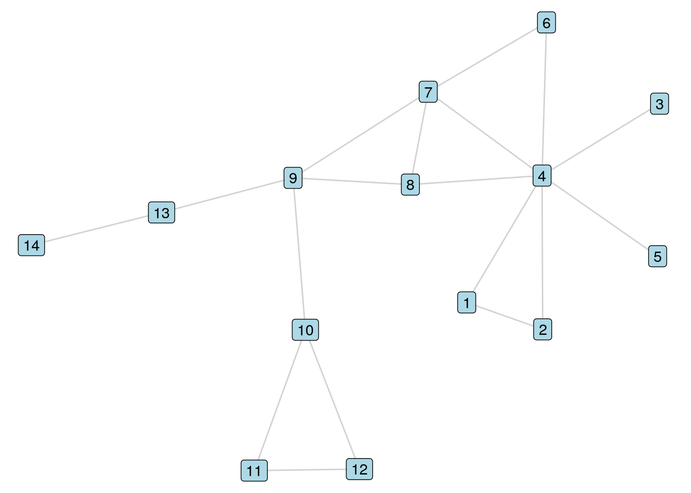
Figure 5.1: The \(G_{14}\) graph

5.1 Theory of graph traversal, paths and distance

5.1.1 Paths and graph traversal

Given any two vertices \(A\) and \(B\) in a graph \(G\), a path between \(A\) and \(B\) is any series of edges in \(G\) that begin at \(A\) and end at \(B\). For example, in our \(G_{14}\) graph, the following are examples of paths between Vertex 9 and Vertex 4:

• \(9 \longleftrightarrow 8 \longleftrightarrow 4\)
• \(9 \longleftrightarrow 7 \longleftrightarrow 4\)
• \(9 \longleftrightarrow 7 \longleftrightarrow 8 \longleftrightarrow 4\)
• \(9 \longleftrightarrow 8 \longleftrightarrow 7 \longleftrightarrow 4\)
• \(9 \longleftrightarrow 7 \longleftrightarrow 6 \longleftrightarrow 4\)
• \(9 \longleftrightarrow 8 \longleftrightarrow 7 \longleftrightarrow 6 \longleftrightarrow 4\)
• \(9 \longleftrightarrow 7 \longleftrightarrow 8 \longleftrightarrow 7 \longleftrightarrow 4\)

A simple path or acyclic path is a path where no vertex is repeated. All except the last path above are simple paths between Vertex 9 and Vertex 4 in \(G_{14}\). In general, because we are interested in efficient paths between vertices, we are only interested in simple paths in a graph. While the number of general paths between two vertices in a graph can be infinite due to possible repeated cycles, the number of simple paths between any two vertices in a graph is always finite. When we refer to a path from now on, we will always mean a simple path unless we say otherwise.

Playing around: Let’s reminisce about Chapter 1 where we studied the Bridges of Königsberg problem. You may recall that an Eulerian path or Euler walk is a path that visits every vertex in a graph at least once and that uses every edge in a graph exactly once. Consider subgraphs of \(G_{14}\) by taking subsets of vertices and the edges that connect them. How many vertices are in the largest subgraph you can form from \(G_{14}\) that contains an Eulerian Path? If you are an R user, you could consider using the eulerian package to verify your answer.

In order to determine whether a path exists between two vertices \(A\) and \(B\) in a graph, we need to be able to search or traverse the graph for possible routes across its edges, starting at Vertex \(A\) and ending at Vertex \(B\), and passing through other vertices as necessary. Let’s take an example from our \(G_{14}\) graph. Let’s say we want to determine if a path exists between Vertex 9 and Vertex 5. When a human looks at a simple graph like this, it is visually obvious that such a path exists. However, as we have mentioned in earlier chapters, most complex graphs cannot be visualized as simply as this one, and computer programs are not human. So we are going to need a more systematic and programmable way of searching the graph for a path from Vertex 9 to Vertex 5.

One option is to traverse the graph using a breadth-first approach. This means that we search all of the immediate neighbors of Vertex 9, then we search the immediate neighbors of the immediate neighbors, and so on until we either eventually find Vertex 5 or until we have covered all vertices and concluded that there is no possible path to Vertex 5. Here is a simple breadth-first algorithm which would achieve this:

1. The immediate neighbors of Vertex 9 are Vertices 7, 8, 10 and 13. We have not found Vertex 5, but we mark Vertex 9 and these neighbor vertices as having been searched.
2. The unsearched immediate neighbors of Vertices 7, 8, 10 and 13 are Vertices 4, 6, 11, 12 and 14. We still have not found Vertex 5, but we add these vertices to the list of vertices which have been searched.
3. The unsearched immediate neighbors of Vertices 4, 6, 11, 12 and 14 are Vertices 1, 2, 3 and 5. We have found Vertex 5 and therefore a path exists between Vertex 9 and Vertex 5.

Alternatively, we could traverse the graph using a depth-first approach. This means that we choose a neighboring vertex of Vertex 9, then find a neighboring vertex of that neighboring vertex, and keep going until we cannot find any more unsearched neighboring vertices. When this happens, we move back a vertex and look for an unsearched neighboring vertex. If we find one, we repeat our process. If not, we move back another vertex and so on until we either find Vertex 5 or we have searched all vertices and conclude that a path to Vertex 5 does not exist. Here is a simple depth-first algorithm which would achieve this:

1. We select Vertex 10 as an immediate neighbor of Vertex 9 and mark both Vertices 9 and 10 as searched.
2. We select Vertex 11 as an unsearched immediate neighbor of Vertex 10 and mark it as searched.
3. We select Vertex 12 as an unsearched immediate neighbor of Vertex 11 and mark it as searched.
4. We cannot find an unsearched immediate neighbor of Vertex 12. So we move back to Vertex 11.
5. We cannot find an unsearched immediate neighbor of Vertex 11. So we move back to Vertex 10.
6. We cannot find an unsearched immediate neighbor of Vertex 10. So we move back to Vertex 9.
7. We select Vertex 8 as an unsearched immediate neighbor of Vertex 9.
8. We select Vertex 4 as an unsearched immediate neighbor of Vertex 8.
9. We select Vertex 3 as an unsearched immediate neighbor of Vertex 4.
10. We cannot find an unsearched immediate neighbor of Vertex 3. So we move back to Vertex 4.
11. We select Vertex 5 as an unsearched immediate neighbor of Vertex 4. We have found Vertex 5 and therefore a path exists between Vertex 9 and Vertex 5.

It appears that the breadth-first approach is quicker and more computationally efficient than the depth-first approach, but this really depends on the specifics of the search. Breadth-first searches like to stay close to the starting node, and gradually increase their search radius. Depth-first searches like to ‘run away and come back’. In our \(G_{14}\) example above, because the network is very small and all nodes are within a short path from Vertex 9, a breadth-first search will usually find the target vertex quickly compared to a depth-first search, whose speed will depend on the route it takes. However, when target nodes are very ‘far away’ in the network, depth-first approaches can be more efficient. On average, however, computation time complexity for both search types is similar⁴⁴.

Thinking ahead: Consider the smallest number of edges that need to be traversed to get from Vertex 9 to Vertex 5 in our \(G_{14}\) graph. Work out what you think that is, and then try to use a depth-first search to move from Vertex 9 to Vertex 5 in different ways. Will the depth-first search always return a path with the smallest number of edges? Why or why not? What about the breadth-first search?

5.1.2 Path length and distance

For a path from vertex \(A\) to vertex \(B\) in a graph, the length of the path is the sum of the weights of the edges traversed in the path. If a graph does not have an edge weight property, then the weight of every edge is assumed to be equal to 1. Therefore, in an unweighted graph, the length of the path is the number of edges traversed on that path.

Looking at the (simple) paths from Vertex 9 to Vertex 4 in \(G_{14}\) as enumerated in Section 5.1.1, we can see that two of the paths have length 2, three of them have length 3, and one has length 4. Now let’s look at a new graph \(G_{14W}\) which has weighted edges as in Figure 5.2.

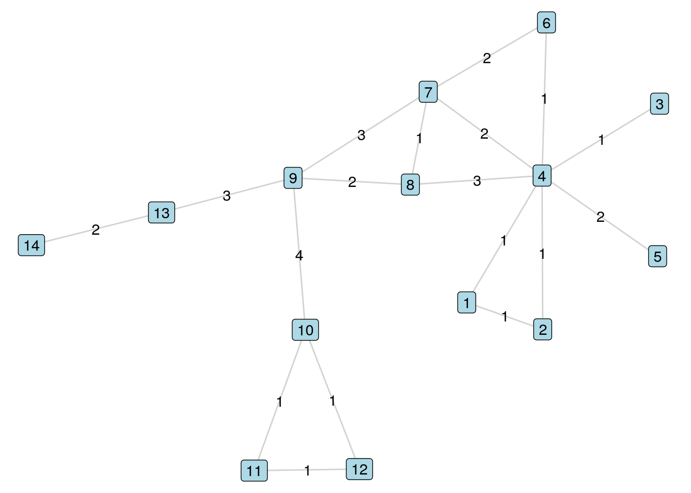
Figure 5.2: The \(G_{14W}\) weighted graph

The list of all simple paths from Vertex 9 to Vertex 4 in \(G_{14W}\) and their lengths are as follows:

• \(9 \longleftrightarrow 8 \longleftrightarrow 4\) (Length 5)
• \(9 \longleftrightarrow 7 \longleftrightarrow 4\) (Length 5)
• \(9 \longleftrightarrow 7 \longleftrightarrow 8 \longleftrightarrow 4\) (Length 7)
• \(9 \longleftrightarrow 8 \longleftrightarrow 7 \longleftrightarrow 4\) (Length 5)
• \(9 \longleftrightarrow 7 \longleftrightarrow 6 \longleftrightarrow 4\) (Length 6)
• \(9 \longleftrightarrow 8 \longleftrightarrow 7 \longleftrightarrow 6 \longleftrightarrow 4\) (Length 6)

The distance between vertices \(A\) and \(B\)—sometimes notated as \(d(A, B)\)—is the length of the shortest path between \(A\) and \(B\). Note that there is no requirement for a unique shortest path, and the shortest path could be traversed in more than one way in a graph. In our unweighted graph \(G_{14}\) the distance between Vertex 9 and Vertex 4 is 2. In the weighted graph \(G_{14W}\) the distance between Vertex 9 and Vertex 4 is 5. If no path exists between \(A\) and \(B\), then the distance is called ‘infinite’ or denoted as \(\infty\) by convention. If \(A\) and \(B\) are vertices of an undirected graph, then \(d(A, B) = d(B, A)\). However, this may not be true for a directed graph.

Distance is an extremely important concept in graphs and has many practical applications. In physical networks like road or rail networks, distance is meant quite literally with greater distances between vertices usually translating to greater time taken or more resources used to traverse between those vertices. In social networks, distance can relate to the ‘familiarity’ or ‘commonality’ between two individuals. Greater distance between individuals in a network usually implies lower likelihood that those individuals know each other in real life, or lower likelihood that information given to one individual will find its way to other individuals. In graphs that represent the knowledge or interests of individuals (such as ‘likes’ in social networks or in knowledge graphs), greater distance between an individual and a topic, event or product usually implies that the individual is less likely to be interested in that topic, event or product. The utility of graph distance measures in fields like transport, communications, marketing, sociology and psychology should therefore be quite obvious.

Distance in weighted graphs needs to be treated with care, particularly in sociological and psychological contexts. Often unweighted distance will be more relevant than weighted distance. For example, if edges are weighted according to the ‘strength’ of a connection between individuals, then the weighted distance between two individuals might be the result of a sequence of multiple edges with low weights, even if those individuals are directly connected by an edge with a higher weight. A simple example of this is in Figure 5.3, where the weighted distance from \(A\) to \(B\) is 2, which arises via the path \(A \longleftrightarrow C \longleftrightarrow B\), despite the fact that \(A\) and \(B\) are adjacent vertices. It is important to understand the meaning of ‘weight’ in your research context before determining if weighted or unweighted distance is appropriate.

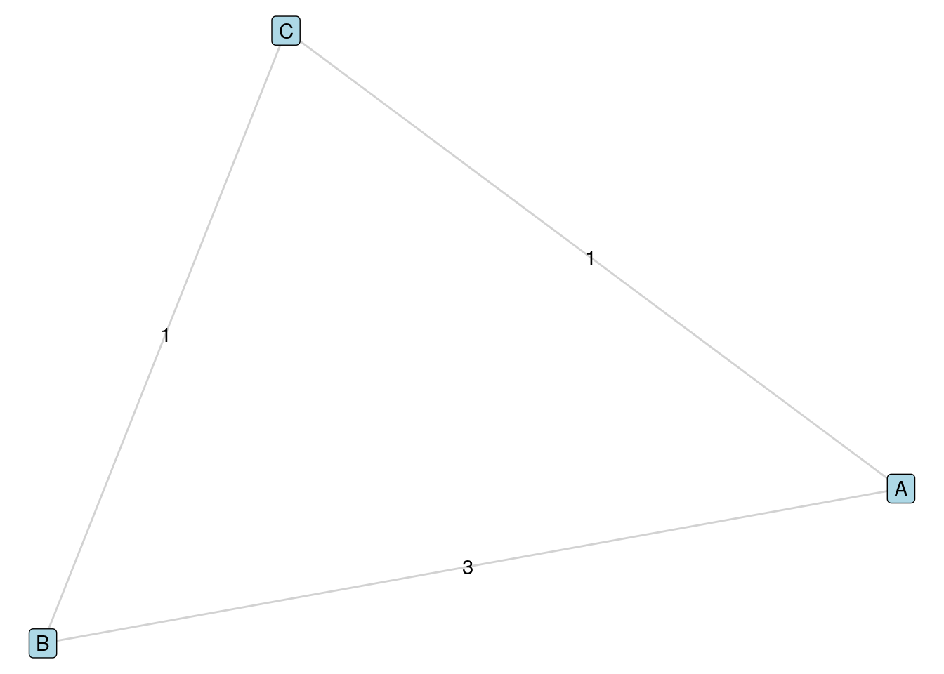
Figure 5.3: Distance needs to be treated with care in weighted graphs. In this case, the weighted distance from \(A\) to \(B\) arises from a path of two edges, even though \(A\) and \(B\) are adjacent in the graph.

5.1.3 Shortest path algorithms

Due to the importance of distance in graphs, various algorithms have been developed to calculate shortest paths. Some of these algorithms—such as Dijkstra’s algorithm or the Bellman-Ford algorithm—focus on a single source shortest path, which calculates the shortest path between a given vertex and all other vertices in the graph. Others—such as Johnson’s algorithm or the Floyd-Warshall algorithm— focus on the all pairs shortest path problem and calculate the shortest path between any pair of vertices in the graph. Special algorithms have also been developed to facilitate fast calculation of shortest path between a specific pair of vertices, such as the A* algorithm.

Dijkstra’s algorithm is perhaps the most well-known (and most established) shortest path algorithm, and the easiest to explain. Let’s take a look at how this algorithm works by using our unweighted \(G_{14}\) graph as an illustrative example. Dijkstra’s algorithm accepts a single initial vertex and calculates the distance between that vertex and all other vertices in the graph. Let’s use Vertex 9 as our initial vertex. Dijkstra’s algorithm operates in a series of iterative steps as follows:

1. We assign a tentative distance between Vertex 9 and itself as zero, and between Vertex 9 and all other vertices as \(\infty\). We then mark Vertex 9 as searched.
2. Move to each of the neighbors of Vertex 9, and calculate the length of the path from Vertex 9 to each of those neighbors and update the tentative distance to this length. In this case, we give a tentative distance of 1 to Vertices 7, 8, 10 and 13. We then mark these vertices as searched.
3. We next go to each of Vertices 7, 8, 10 and 13 in turn, marking each one as current as we proceed. For each current vertex, we calculate the length of the shortest path from Vertex 9 to each of the unsearched neighbors of the current vertex which pass through the current vertex. If that length is smaller than the existing tentative distance, update the tentative distance with this length. If we move to Vertex 7 first, we see two unsearched neighbors: Vertices 4 and 6. The distance from Vertex 9 to both these vertices passing through Vertex 7 is 2, which is less than \(\infty\), and so we update the tentative distances from Vertex 9 to Vertices 4 and 6 to 2.
4. In a similar fashion we update the tentative distances from Vertex 9 to Vertices 11, 12 and 14 to 2.
5. We mark Vertices 4, 6, 11, 12 and 14 as searched and move to these vertices as current vertices and repeat the process for their neighbors. In this way, we update the tentative distance from Vertex 9 to Vertices 1, 2, 3 and 5 to 3. We mark Vertices 1, 2, 3 and 5 as searched.
6. We have now searched all vertices in the graph, and the tentative distances between Vertex 9 and all other vertices are now assigned as the final distances.

Playing around: Try to repeat the process of Dijkstra’s algorithm for the weighted graph \(G_{14W}\). Which vertex has the shortest distance from Vertex 9 and which vertex has the longest distance?

Single source shortest path algorithms like Dijkstra’s algorithm can be used to solve the all pairs distance problem by simply repeating the algorithm for each vertex in the graph. For large graphs, however, this can be inefficient, which explains why alternative algorithms have been developed for the all pairs problem⁴⁵.

5.1.4 Graph diameter and density

The diameter of a graph \(G\) is the maximum distance between any pair of vertices in \(G\). Alternatively stated, it is the longest shortest path between vertices in \(G\). If a graph is not a connected graph, then by definition its diameter is infinite. Diameter is usually only a useful measure in connected graphs, or in studying connected subgraphs of larger graphs.

The diameter of a social network is an intuitive measure of the overall ‘closeness’ of the individuals in that network. Networks with smaller diameters can often be considered as more ‘close-knit’ communities. However, care needs to be taken in interpreting the diameter of a network, particularly given that other measures may be more representative of how close-knit a community is. Common alternative metrics used to assess overall network ‘closeness’ include:

• Average distance between all pairs of vertices
• The density of the network, which is defined as the number of edges divided by the total possible number of edges in a graph⁴⁶. A complete graph, for example, would have a density of 1. Graphs with lower density are called sparse graphs.

Consider the two graphs in Figure 5.4. In the first graph, the diameter is 5, and in the second the diameter is 4. However, the average distance between vertices in the first graph is 2.38, and in the second graph it is 2.49. Both graphs have the same density of 0.2. Therefore, one measure would regard the first graph as ‘closer’, another would regard the second graph as closer, and the third measure would regard them as the same.

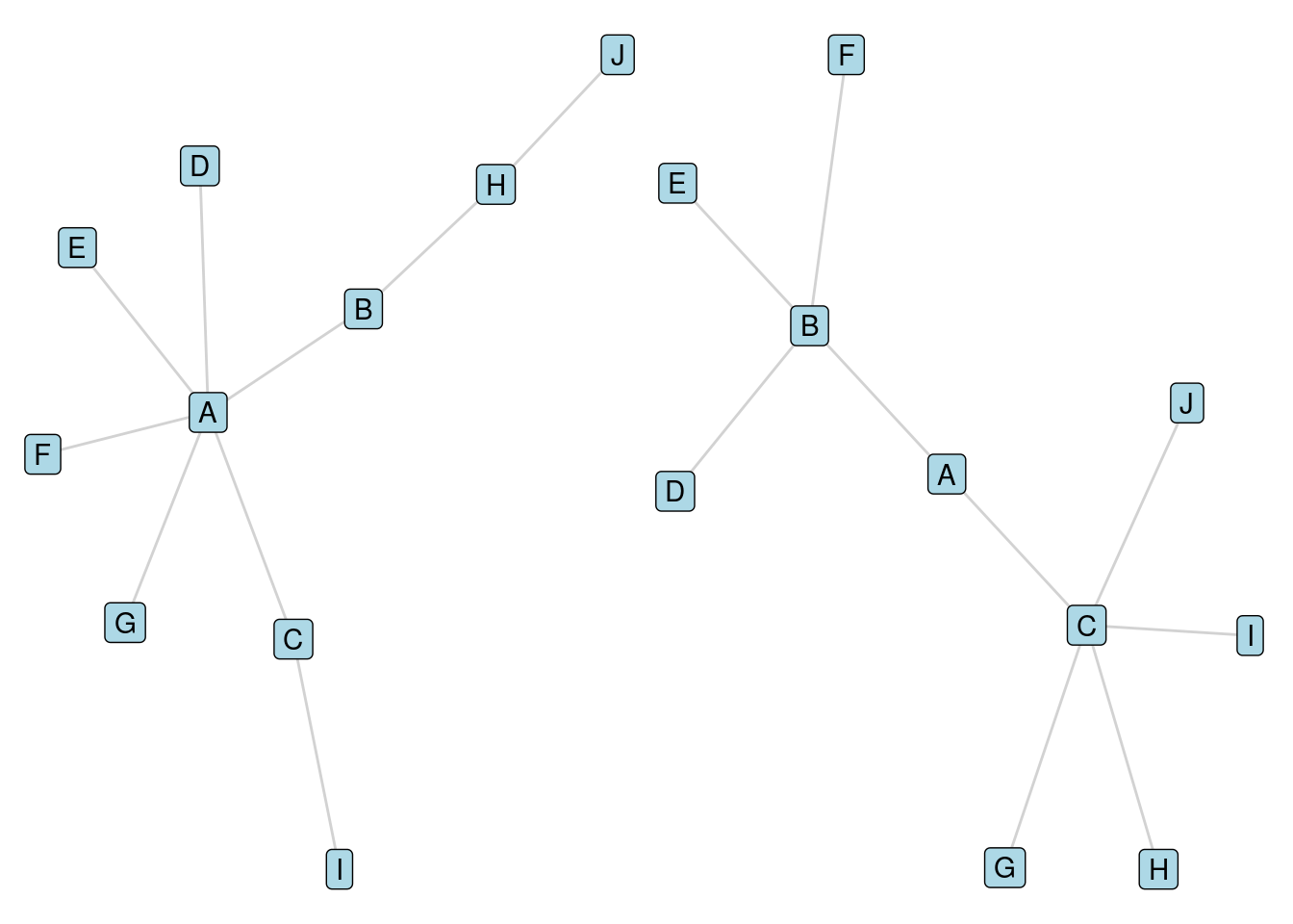
Figure 5.4: Two graphs illustrating how closeness can be measured in different ways

Playing around: Graph distance and diameter is of great interest in everyday life. You may know the theory of the six degrees of separation, which suggests that the entire world is a connected graph where the distance between any two people is at most 6. Alternatively stated, the world is a connected graph with a diameter of no more than 6. Several industry-specific case studies of this have arisen for research and just for fun. The first was a 1969 paper by two psychologists (Travers & Milgram (1969)), which used an experiment of chain letters to determine that the average distance between people in a population in Nebraska and Massachusetts was 6.2. A 2011 study of the Facebook graph (Ugander et al. (2011)) determined that the Facebook member network was almost fully connected with 99.91% of vertices in a connected subgraph, and that the average distance between vertices was 4.7. In the entertainment industry, the Bacon number is used to denote the distance between an individual and the actor Kevin Bacon, based on participation in the same movie or TV production. In academia, the Erdös number is used to denote the distance between an individual and the mathematician Paul Erdös. Both Bacon and Erdös have arisen as central points because they were highly active in their disciplines and as a result have high centrality in their network. We will look at centrality in the next chapter, but if you are interested you can find the Bacon number of any actor by visiting https://oracleofbacon.org/.

5.2 Calculating paths, distance, diameter and density

5.2.1 Calculating in R

Thanks to packages like igraph in R, it is much easier to calculate path, distance and density metrics than to understand the theory behind them. In this section we will illustrate various functions that can be used to easily calculate these metrics. Before we begin, let’s create the graphs \(G_{14}\) and \(G_{14W}\) from the previous section by loading the g14_edgelist data set from the onadata package or by downloading it from the internet⁴⁷.

# download the edgelist
g14_edgelist <- read.csv("https://ona-book.org/data/g14_edgelist.csv")

# view head
head(g14_edgelist)

##   from to weight
## 1    9 10      4
## 2   10 11      1
## 3   11 12      1
## 4   10 12      1
## 5    9 13      3
## 6   13 14      2

Let’s start by creating the weighted \(G_{14W}\) graph from the previous section.

# create weighted graph
(g14w <- igraph::graph_from_data_frame(g14_edgelist, directed = FALSE))

## IGRAPH 065b116 UNW- 14 18 -- 
## + attr: name (v/c), weight (e/n)
## + edges from 065b116 (vertex names):
##  [1] 9 --10 10--11 11--12 10--12 9 --13 13--14 9 --8  9 --7  8 --7  4 --6  4 --7  8 --4  6 --7  4 --1  4 --2  4 --3 
## [17] 4 --5  1 --2

The all_simple_paths() function in igraph returns all paths from a specified vertex, and expects at least an igraph object and a vertex name for the from vertex as arguments. If the to argument specifies a vertex, then the function will return only paths between the from and to vertices. Otherwise, it will return a list containing all paths from the specified vertex to all other vertices. Note that these functions expect the vertex name as a character string.

igraph::all_simple_paths(g14w, from = "9", to = "4")

## [[1]]
## + 3/14 vertices, named, from 065b116:
## [1] 9 8 4
## 
## [[2]]
## + 4/14 vertices, named, from 065b116:
## [1] 9 8 7 4
## 
## [[3]]
## + 5/14 vertices, named, from 065b116:
## [1] 9 8 7 6 4
## 
## [[4]]
## + 4/14 vertices, named, from 065b116:
## [1] 9 7 8 4
## 
## [[5]]
## + 3/14 vertices, named, from 065b116:
## [1] 9 7 4
## 
## [[6]]
## + 4/14 vertices, named, from 065b116:
## [1] 9 7 6 4

We see that this agrees with our manual calculations in Section 5.1.1 and is the same whether or not the edges are weighted. This function is easy to use in the case of undirected graphs. When using with digraphs, there is an additional argument called mode, specifying the direction of the paths you are seeking. out, in, all or total are the accepted values for this argument.

The all_shortest_paths() function performs the same task as the previous function but restricts the output to paths of the shortest length. This function returns a list of objects, but the paths can be found in the res element of the list.

shortest_9to4 <- igraph::all_shortest_paths(g14w, from = "9", to = "4")
shortest_9to4$res

## [[1]]
## + 3/14 vertices, named, from 065b116:
## [1] 9 8 4
## 
## [[2]]
## + 3/14 vertices, named, from 065b116:
## [1] 9 7 4
## 
## [[3]]
## + 4/14 vertices, named, from 065b116:
## [1] 9 8 7 4

Note that the function has returned the shortest path according to edge weights. To ignore edge weights, simply set weights = NA. This is equivalent to calculating shortest paths in our unweighted \(G_{14}\) graph.

shortest_9to4_uw <- igraph::all_shortest_paths(g14w, 
                                               from = "9", to = "4", 
                                               weights = NA)
shortest_9to4_uw$res

## [[1]]
## + 3/14 vertices, named, from 065b116:
## [1] 9 7 4
## 
## [[2]]
## + 3/14 vertices, named, from 065b116:
## [1] 9 8 4

The distances() function calculates distance in a graph. By default, it calculates the distance between all pairs of vertices and returns the results as a distance matrix.

distances(g14w)

##    9 10 11 13 8  4  6  1 12 14 7  2  3  5
## 9  0  4  5  3 2  5  5  6  5  5 3  6  6  7
## 10 4  0  1  7 6  9  9 10  1  9 7 10 10 11
## 11 5  1  0  8 7 10 10 11  1 10 8 11 11 12
## 13 3  7  8  0 5  8  8  9  8  2 6  9  9 10
## 8  2  6  7  5 0  3  3  4  7  7 1  4  4  5
## 4  5  9 10  8 3  0  1  1 10 10 2  1  1  2
## 6  5  9 10  8 3  1  0  2 10 10 2  2  2  3
## 1  6 10 11  9 4  1  2  0 11 11 3  1  2  3
## 12 5  1  1  8 7 10 10 11  0 10 8 11 11 12
## 14 5  9 10  2 7 10 10 11 10  0 8 11 11 12
## 7  3  7  8  6 1  2  2  3  8  8 0  3  3  4
## 2  6 10 11  9 4  1  2  1 11 11 3  0  2  3
## 3  6 10 11  9 4  1  2  2 11 11 3  2  0  3
## 5  7 11 12 10 5  2  3  3 12 12 4  3  3  0

Again, specific subsets of vertices can be selected and the function will return a matrix for just those subsets, and the same mode argument can be used for digraphs. Weights can be ignored by setting weights = NA. The algorithm used to calculate the shortest path is automatically selected, but can be specified using the algorithm argument.

distances(g14w, v = "9", to = "4", weights = NA, 
          algorithm = "bellman-ford")

##   4
## 9 2

The mean_distance() function calculates the average distance between all pairs of vertices. Note that this function does not consider edge weights.

mean_distance(g14w)

## [1] 6.208791

To consider edge weights in calculating average distance, you should take the mean of the off-diagonal elements of the distance matrix. This is most easily done by extracting the lower and upper triangles of the distance matrix.

# get lower and upper triangles of weighted distance matrix 
dist <- distances(g14w)
off_diag_dist <- dist[upper.tri(dist) | lower.tri(dist)] 

# calcuate mean
mean(off_diag_dist)

## [1] 6.208791

Graph diameter can be calculated using the diameter() function and is equal to the maximal element of the distance matrix. Again, weights can be ignored by setting weights = NA.

diameter(g14w)

## [1] 12

If a graph is not connected, the diameter() function will return the diameter of the largest connected component by default. The function farthest_vertices() will return a pair vertices at either end of a diameter path, and the function get_diameter() will return a full diameter path.

farthest_vertices(g14w, weights = NA)

## $vertices
## + 2/14 vertices, named, from 065b116:
## [1] 11 1 
## 
## $distance
## [1] 5

get_diameter(g14w, weights = NA)

## + 6/14 vertices, named, from 065b116:
## [1] 11 10 9  8  4  1

Finally, the edge_density() function will calculate the density of the graph. You can find the formula for edge density in an earlier footnote in this chapter and, if you like, you can verify this manually for our \(G_{14W}\) graph.

edge_density(g14w)

## [1] 0.1978022

Playing around: The distance() function in igraph allows you to select from three algorithms to use: Dijkstra, Bellman-Ford and Johnson. If you are interested in computation speed, you could try an experiment on a large graph to see which one is faster. The microbenchmark package in R is useful for running a computation many times and benchmarking its average speed. You could try creating a directed graph from the wikivote data set in the onadata package or via the internet⁴⁸, calculating the distance matrix using each of the three algorithms and benchmarking the speed. I found the Johnson algorithm to be about four times faster than the others. Don’t try this, however, if you are on a low memory or slow CPU computer.

5.2.2 Calculating in Python

The functions for path, distance, density and diameter in the networkx package in Python are very similar to those in igraph in R. First, let’s load our weighted graph \(G_{14W}\).

import networkx as nx
import pandas as pd

g14w_edges = pd.read_csv("https://ona-book.org/data/g14_edgelist.csv")

g14w = nx.from_pandas_edgelist(g14w_edges, source = "from", 
target = "to", edge_attr = True)

To calculate all simple paths between two specified nodes, use the all_simple_paths() function.

simple_paths = nx.all_simple_paths(G = g14w, source = 9, target = 4)
[path for path in simple_paths]

## [[9, 8, 7, 4], [9, 8, 7, 6, 4], [9, 8, 4], [9, 7, 8, 4], [9, 7, 4], [9, 7, 6, 4]]

To calculate all shortest paths between two specified nodes, use the all_shortest_paths() function. By default, this will ignore edge weights.

shortest_paths_uw = nx.all_shortest_paths(G = g14w, source = 9, 
target = 4)
[path for path in shortest_paths_uw]

## [[9, 8, 4], [9, 7, 4]]

To consider edge weights, use the name of the weight attribute as the value of the weight argument.

shortest_paths_w = nx.all_shortest_paths(G = g14w, source = 9, 
target = 4, weight = 'weight')
[path for path in shortest_paths_w]

## [[9, 8, 4], [9, 7, 4], [9, 8, 7, 4]]

For undirected graphs, the shortest_path() function will calculate a single shortest path for every pair of vertices in the graph, returning the paths in a dict. You can also specify source and target node subsets.

shortest_paths_from9 = nx.shortest_path(g14w, source = 9, 
weight = 'weight')

# view one path to vertex 11
shortest_paths_from9.get(11)

## [9, 10, 11]

For directed graphs, various algorithm-specific functions are available, such as dijkstra_path(), bellman_ford_path() and many others.

Distances can be calculated using the shortest_path_length() function, either to produce all distances or to focus on a specific source and/or target. This will return a dict if a single source or target is provided, or a tuple otherwise.

distances_from9 = nx.shortest_path_length(g14w, source = 9, 
weight = 'weight')
distances_from9

## {9: 0, 8: 2, 13: 3, 7: 3, 10: 4, 4: 5, 14: 5, 6: 5, 11: 5, 12: 5, 1: 6, 2: 6, 3: 6, 5: 7}

Average distance can be calculated using the average_shortest_path_length() function. Include weights as an argument to get the average weighted distance.

nx.average_shortest_path_length(g14w, weight = 'weight')

## 6.208791208791209

Diameter can be calculated using the diameter() function, but this will only compute the unweighted diameter.

nx.diameter(g14w)

## 5

To calculate the weighted diameter, simply take the maximum value of the weighted distances across all pairs.

distances = nx.shortest_path_length(g14w, weight = 'weight')
max([max(distance[1].values()) for distance in distances])

## 12

Finally, edge density can be calculated using the density() function.

nx.density(g14w)

## 0.1978021978021978

5.3 Examples of uses

To illustrate uses of paths and distance in organizational settings, we will go through a couple of examples. We will look at real data from the workfrance graph which we introduced earlier in Section 3.1.3. The workfrance data set contains information captured in an experimental study in an office building in France. Vertices in this data set represent individual employees, and edges exist between employees if they have spent a minimum amount of time together in the same place in the building. Let’s download the data and create the graph in R.

set.seed(123)

# download workfrance data sets
workfrance_edges <- read.csv(
    "https://ona-book.org/data/workfrance_edgelist.csv"
)
workfrance_vertices <- read.csv(
    "https://ona-book.org/data/workfrance_vertices.csv"
)

# create graph
(workfrance <- igraph::graph_from_data_frame(
    d = workfrance_edges,
    vertices = workfrance_vertices,
    directed = FALSE
))

## IGRAPH 4e41742 UN-- 211 932 -- 
## + attr: name (v/c), dept (v/c), mins (e/n)
## + edges from 4e41742 (vertex names):
##  [1] 3   --159  253 --3    3   --447  3   --498  3   --694  3   --751  3   --859  3   --908  14  --18   99  --14  
## [11] 14  --441  520 --14   14  --544  14  --653  14  --998  15  --120  15  --160  15  --162  15  --178  15  --259 
## [21] 15  --261  15  --295  15  --353  15  --372  15  --464  15  --491  15  --498  15  --909  15  --1090 39  --18  
## [31] 99  --18   429 --18   488 --18   527 --18   18  --621  18  --650  753 --18   18  --797  18  --845  99  --27  
## [41] 160 --27   259 --27   295 --27   27  --346  27  --1392 34  --156  34  --250  34  --259  34  --489  34  --615 
## [51] 34  --694  34  --884  34  --959  219 --38   38  --435  39  --71   39  --72   39  --99   118 --39   39  --219 
## [61] 39  --339  39  --407  39  --468  39  --871  39  --939  43  --285  43  --339  43  --809  43  --866  43  --985 
## [71] 118 --47   47  --366  47  --691  54  --74   54  --134  54  --158  54  --236  55  --110  55  --164  447 --55  
## + ... omitted several edges

We have built a graph with 211 vertices and 932 edges. The vertices have a dept property which indicates the department the person works in, and the edges have a mins property which indicates the number of minutes spent together in the same place. The mins property could be considered a measure of how strong the connection between two individuals is, so let’s make it a weight in the graph.

E(workfrance)$weight <- E(workfrance)$mins

5.3.1 Facilitating introductions in a workplace

A simple use case of shortest paths is to help connect individuals via common connections or intermediaries. Let’s take two vertices from our workfrance graph who are from different departments. Let’s select Vertices 3 and 55. Let’s see what departments they are in.

V(workfrance)$dept[V(workfrance)$name %in% c("3", "55")]

## [1] "DMI" "SSI"

Now let’s determine the unweighted distance between these two employees in the network.

distances(workfrance, v = "3", to = "55", weights = NA)

##   55
## 3  2

These two individuals have an unweighted distance of 2 in the network, meaning they can connect through one intermediary. Now we can use our all_shortest_paths() function to determine who the common intermediary is.

all_shortest_paths(workfrance, from = "3", to = "55", weight = NA)$res 

## [[1]]
## + 3/211 vertices, named, from 4e41742:
## [1] 3   447 55

There is one common intermediary: employee 447. Therefore, if employees 3 and 55 do not know each other, employee 447 may be able to introduce them. Note that there may be more than one suggestion for intermediaries. For example:

(paths <- all_shortest_paths(workfrance, from = "3", to = "290", 
                             weight = NA)$res)

## [[1]]
## + 3/211 vertices, named, from 4e41742:
## [1] 3   859 290
## 
## [[2]]
## + 3/211 vertices, named, from 4e41742:
## [1] 3   694 290

In this case, we could consider using the edge weights to rank the intermediary options, on the basis that higher weights may indicate stronger connections. Let’s visualize these two options by looking at the subgraph with edge weights in Figure 5.5.

subgraph <- induced_subgraph(workfrance, 
                             vids = c("3", "290", "694", "859"))

ggraph(subgraph) +
    geom_edge_link(aes(edge_width = weight, label = weight), 
                   color = "grey", alpha = 0.7, 
                   show.legend = FALSE) +
    geom_node_label(size = 3, fill = "lightblue", aes(label = name)) +
    theme_void()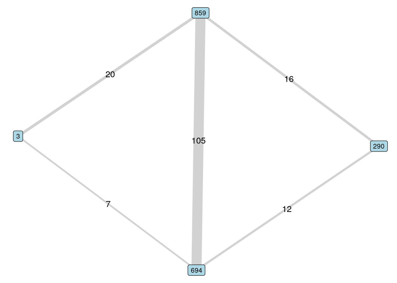

Figure 5.5: Selecting an intermediary according to higher edge weights

Here we may recommend employee 859 first on the basis of higher edge weights and therefore possibly greater familiarity with employees 3 and 290.

Playing around: You may have seen this kind of ‘introduction’ system at work through social networks such as LinkedIn, which can suggest how to be introduced to another member via a common connection. You may also have seen the distance of an individual from you in the network, with direct connections (distance of 1) labelled as 1st, connections of connections (distance of 2) labelled as 2nd, and so on. These huge networks rarely calculate distances of greater than 3 or suggest connection paths with more than one intermediary because of the massive computational cost of doing so. If you have a LinkedIn profile, you may want to go and explore your second order connections and view the intermediaries who can connect you. This is the equivalent of looking at all the shortest paths between you and that individual in the network.

5.3.2 Finding distant colleagues in a workplace

Now, imagine that a professional event is being organized in the office building in France, where employees will be assigned to one of 21 tables of ten people⁴⁹. You have been asked to try to help ensure that the tables contain a good mix of individuals and to avoid tables where everyone knows each other very well.

Before we start, we should check whether this graph has any disconnected components.

is.connected(workfrance)

## [1] TRUE

So there are no disconnected components in this graph. Let’s also look at the diameter of this graph to get a sense of the maximum possible distance between any pair of individuals.

diameter(workfrance, weights = NA)

## [1] 6

As a first step, we can pick 21 people who have an unweighted distance of 1 from each other and sit them all at a different table. That would certainly be a good starting point. We can use the neighbors() function in igraph and look for a vertex that has the most neighbors⁵⁰.

# create vectors to capture name and no of neighbors
v_name <- c()
n_neighbors <- c()

# capture name and no of neighbors for every vertex
for (v in V(workfrance)$name) {
    v_name <- append(v_name, v)
    n_neighbors <- append(n_neighbors, 
                          length(neighbors(workfrance, v)))
}

# find the max
v_name[which.max(n_neighbors)]

## [1] "603"

It looks like employee 603 has the most neighbors. Let’s find out how many.

n_neighbors[which.max(n_neighbors)]

## [1] 28

We could pick any 20 from the neighbors of employee 603 and that would be a great starting point for our 21 tables. Let’s pick those with the highest mins property (assuming that this represents a closer relationship). We can use the inc() function to get all edges containing employee 603 and then select those that have the highest mins property.

edges603 <- E(workfrance)[inc("603")]
sort603_mins <- sort(edges603$mins, decreasing = TRUE)
(top_edges603 <- edges603[order(sort603_mins)][1:20])

## + 20/932 edges from 4e41742 (vertex names):
##  [1] 603--1392 603--1323 603--1362 859--603  603--954  603--1245 603--779  603--649  691--603  694--603  706--603 
## [12] 603--725  487--603  420--603  428--603  387--603  401--603  603--272  290--603  346--603

Now we have the ‘closest’ 20 people to employee 603. Let’s create an edge subgraph and extract the vertices.

subgraph603 <- igraph::subgraph.edges(workfrance, eid = top_edges603)
V(subgraph603)$name

##  [1] "290"  "420"  "428"  "691"  "706"  "694"  "859"  "346"  "387"  "401"  "487"  "603"  "649"  "725"  "779"  "954" 
## [17] "1245" "1323" "1362" "1392" "272"

We can also look at the departments of these individuals:

V(subgraph603)$dept

##  [1] "DG"   "DISQ" "DISQ" "DISQ" "DMCT" "DMI"  "DMI"  "DST"  "DST"  "DST"  "DST"  "DST"  "DST"  "DST"  "DST"  "DST" 
## [17] "DST"  "DST"  "DST"  "DST"  "SRH"

We see some considerable department similarity, which makes sense. Now that we have found the first person for each table, we will want to try to make sure that we sit that person with nine other people who have some distance from them, and to minimize neighbors sitting at the same table. Let’s start with our first employee 603, and call this Table 1. Because there are only 21 tables but employee 603 has 28 neighbors, we might be willing to allow one neighbor to sit at Table 1. Let’s sit them with the neighbor with whom they spent the least minutes.

edges603[which.min(edges603$mins)]

## + 1/932 edge from 4e41742 (vertex names):
## [1] 77--603

So we will sit employee 603 with employee 77. Now we can select a third individual who has a reasonable distance in the network from both employee 603 and employee 77. Let’s look at all these distances.

(distance603_77 <- distances(workfrance, v = c("603", "77"), 
                             weights = NA))

##     89 97 118 220 378 656 720 741 886 1204 1209 1492 290 502 47 119 198 213 253 267 270 343 366 420 428 445 478 520 525
## 603  3  2   2   2   3   3   3   2   3    2    3    4   1   4  2   2   2   2   2   1   2   2   2   1   1   2   2   2   2
## 77   2  1   2   1   2   2   2   2   2    1    2    3   2   4  3   3   3   3   3   2   3   3   3   2   2   3   3   3   2
##     660 691 836 39 43 59 63 72 80 122 211 219 246 257 285 339 407 466 468 533 702 706 753 784 790 793 809 866 871 889
## 603   2   1   2  2  3  3  3  2  2   2   3   3   2   2   3   2   2   3   2   4   3   1   2   2   3   3   3   3   3   2
## 77    3   2   3  3  3  3  2  2  3   1   3   3   3   3   3   3   2   3   3   3   4   2   2   3   3   3   3   3   3   2
##     894 923 939 3 15 34 54 74 79 99 120 131 134 141 156 158 159 160 162 165 178 183 193 205 236 242 250 259 261 295 333
## 603   2   2   3 2  3  2  3  2  3  1   2   3   3   2   2   3   2   2   2   4   3   2   3   3   2   4   3   2   2   2   2
## 77    3   3   2 2  2  2  2  1  2  2   2   3   3   2   2   2   1   2   1   3   3   2   2   3   3   3   2   1   2   2   2
##     353 372 425 447 453 460 464 489 491 498 574 615 642 677 694 751 763 859 880 884 909 959 1067 1090 1164 1238 1342 38
## 603   3   2   4   3   2   3   3   3   3   3   3   3   3   3   1   3   3   1   3   3   2   3    2    3    2    3    2  4
## 77    2   2   3   3   2   3   2   2   2   2   2   2   2   4   2   2   2   2   2   2   3   2    2    3    3    2    1  3
##     172 184 210 222 248 252 269 275 322 374 424 465 477 486 504 510 513 527 577 634 638 674 743 771 867 882 893 908 921
## 603   3   3   1   3   3   2   3   2   3   3   2   3   3   3   3   3   3   3   3   2   3   3   2   3   3   2   3   2   3
## 77    4   4   2   4   4   3   4   3   3   4   3   4   4   3   4   4   4   3   4   3   4   4   3   4   4   3   4   3   3
##     1485 27 71 77 147 215 346 387 401 426 429 487 488 580 582 603 649 725 779 954 1245 1323 1362 1392 14 181 441 544
## 603    2  2  1  1   1   1   1   1   1   2   2   1   2   2   2   0   1   1   1   1    1    1    1    1  2   2   3   3
## 77     3  2  2  0   2   1   1   2   2   2   1   2   2   2   2   1   1   2   2   2    2    2    2    2  3   3   4   4
##     778 998 1260 106 245 435 440 117 197 200 413 432 461 475 496 626 653 874 977 1414 18 232 272 531 621 650 744 797
## 603   3   3    3   3   3   3   2   1   3   2   2   3   2   2   3   3   2   2   3    2  2   2   1   2   3   2   2   2
## 77    3   4    4   3   3   2   2   2   3   3   3   3   3   3   4   4   2   3   4    3  2   3   2   3   3   3   3   3
##     845 55 110 164 173 628 970 985
## 603   2  2   3   3   3   2   4   3
## 77    3  3   4   3   3   2   4   2

We could use the mean of the distances to decide on the person with the furthest distance from those already selected.

which.max(colMeans(distance603_77))

## 502 
##  14

We can select employee 502 for the third seat, and we iterate to find the remainder of the people at the table. In this iteration, we make sure that the same person does not arise twice in the calculations.

table1 <- c("603", "77", "502")

# complete remainder of table
for (i in 4:10) {
    # get distances from already chosen table members
    dists <- distances(workfrance, v = table1, weights = NA) 
    # get vertices with maximum mean distance excluding already chosen
    new <- dists |>
        as.data.frame() |> 
        subset(select = !(colnames(dists) %in% table1)) |> 
        colMeans() |> 
        which.max() |> 
        names()
    # add first of these to table
    table1[i] <- new[1]
}

# view complete table 1
table1

##  [1] "603" "77"  "502" "533" "496" "970" "165" "677" "977" "38"

Now let’s assign a table property to the workfrance graph and take a look at where our members of Table 1 appear, as in Figure 5.6.

# add a table property to workfrance graph
V(workfrance)$table <- ifelse(
    V(workfrance)$name %in% table1, "1", "2-21"
)

# visualize
set.seed(123)
ggraph(workfrance, layout = "fr") +
    geom_edge_link(color = "grey", alpha = 0.7) +
    geom_node_point(size = 4, aes(color = as.factor(table))) +
    labs(color = "Table") +
    theme_void()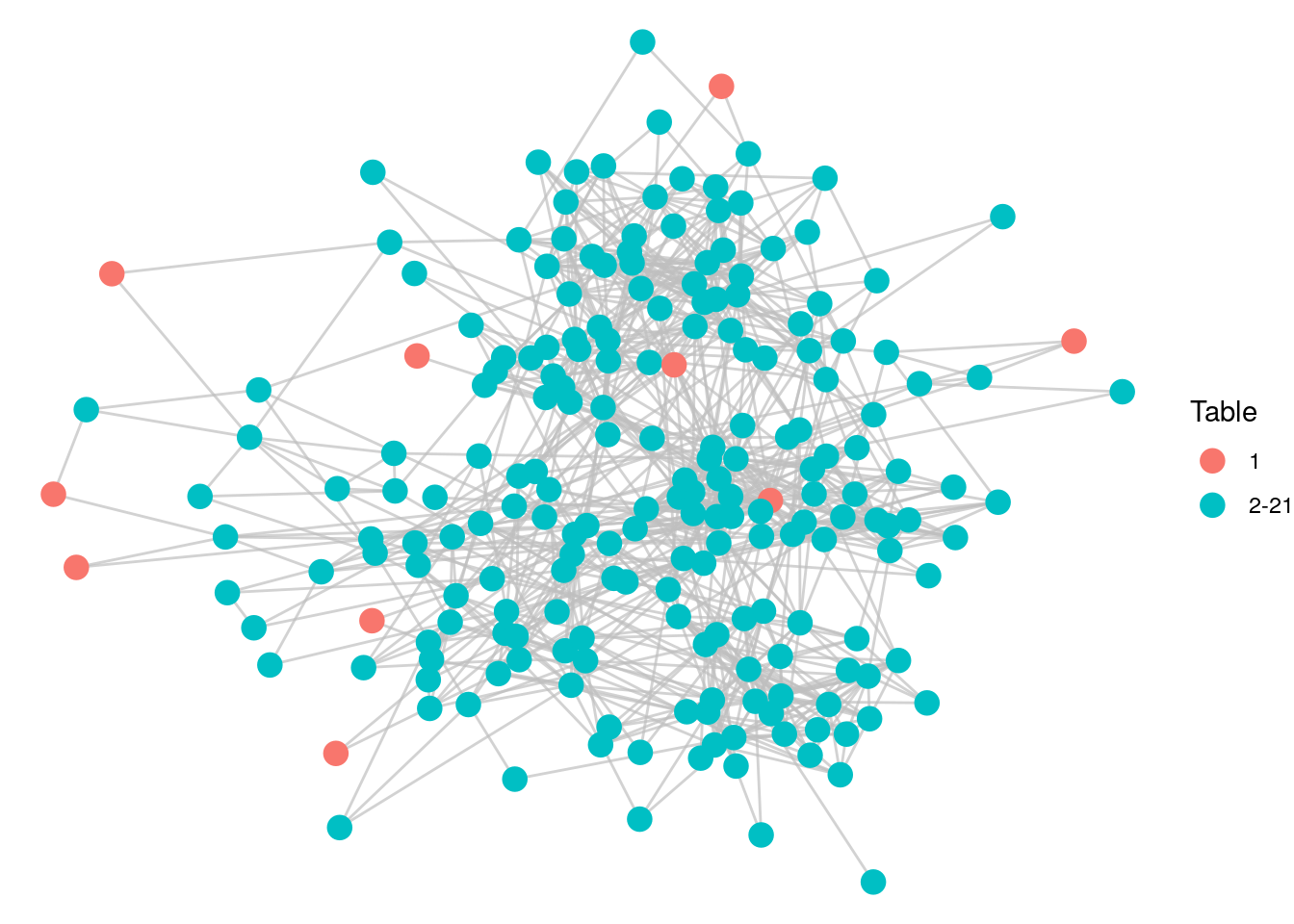

Figure 5.6: Individuals selected for Table 1 based on optimizing for distance

It looks as if we have done a good job of maximizing for distance in the network in our Table 1 selection. Let’s check the average distance among the employees at Table 1.

mean(distances(workfrance, v = table1, to = table1, weights = NA))

## [1] 3.96

Given that the diameter of the graph is 6, and that we decided to include a pair of individuals with a distance of 1 on this table, a mean distance of 3.96 seems pretty good. Let’s look at the department mix of our ten people at Table 1.

V(workfrance)$dept[V(workfrance)$name %in% table1]

##  [1] "DG"   "DMCT" "DMI"  "DMI"  "DSE"  "DST"  "DST"  "SFLE" "SFLE" "SSI"

We have seven departments represented at a table of ten, which seems another good indication of a diverse table. This gives you a sense of how you can use paths and distance as a mathematical model for familiarity in a network. If you are interested in continuing this process to fill further tables, see the exercises at the end of this chapter.

5.4 Learning exercises

5.4.1 Discussion questions

1. Define what is meant by graph traversal and describe why it is an important topic in network analysis.
2. Describe what is meant by a path, a simple path and a shortest path. Provide examples of each using the \(G_{14}\) and the \(G_{14W}\) graph.
3. Describe the difference between a breadth-first and a depth-first graph search algorithm. Name an example of each.
4. Define the distance between two vertices in a graph. Using \(G_{14}\) or \(G_{14W}\), give an example of vertices which have a distance of 3, and list all shortest paths between those vertices.
5. Define the diameter of a connected graph. List a path whose distance is equal to the diameter of \(G_{14}\).
6. Define the density of a graph. What does it mean for a graph to be sparse?
7. If a graph \(G\) has four vertices \(A\), \(B\) , \(C\), and \(D\), and its only edges are from \(A\) to all other vertices, calculate the density of \(G\).
8. Write down a procedure to describe how Dijkstra’s algorithm would calculate all shortest paths from Vertex 7 in \(G_{14}\).
9. Manually determine all simple paths and all shortest paths between Vertices 1 and 13 in \(G_{14}\).
10. Manually determine all shortest weighted paths between Vertices 1 and 13 in \(G_{14W}\).

5.4.2 Data exercises

1. Use appropriate functions to determine all simple paths and all shortest paths between Vertices 1 and 13 in \(G_{14}\) and check that the output agrees with your manual calculation in Discussion Question 9.
2. Use appropriate functions to determine all shortest weighted paths between Vertices 1 and 13 in \(G_{14W}\) and check that the output agrees with your manual calculation in Discussion Question 10.
3. Create a subgraph of \(G_{14W}\) consisting only of vertices 6 through 14. Use an appropriate procedure to calculate the unweighted and weighted distances between all pairs of vertices in this subgraph.
4. Calculate the unweighted and weighted diameter of the subgraph from the previous exercise, and calculate its density.

For Exercises 5 to 7, load the friends_tv_edgelist data set from the onadata package or download it from the internet⁵¹. This is a full network of all characters appearing in every season of the Friends TV series based on characters speaking in the same scene together. Each edge has a weight according to the number of scenes those characters both spoke in together, but ignore this for this set of exercises and simply create an unweighted, undirected graph from this edgelist.

5. Check whether the Friends network is connected and calculate the diameter of the network. Find a path with length equal to the diameter. The diameter is surprisingly small for a network of this size. Why might this be?
6. Find all simple paths from Billy Crystal to Mr Bing and from Janice to Mrs Bing. Try to calculate what proportion of the connections have distance 2 in this graph. The results may help with the answer to the previous question.
7. Calculate the density of the network. Create a subgraph consisting of the six main characters: Monica, Chandler, Phoebe, Ross, Rachel and Joey. Calculate the density of this subgraph. What term would you use to describe this subgraph?
8. A ‘clique’ in a graph is a subgraph which is complete (that is, all vertices are connected to each other and the density is 1). Can you find a clique in the Friends graph that does not contain any of the main characters⁵²?
9. Create a new subgraph by removing the six main characters from the original graph. Check whether this subgraph is connected. What can you conclude from this?
10. Calculate the largest diameter of connected components of this new graph. Find the pair of characters associated with this diameter path. Find the largest clique in this graph.
11. Extension: Extend the example in Section 5.3.2 by creating a second table for the event. Remember that this second table cannot include anyone selected for Table 1. Explore your results by visualizing them and analyzing the average distance for Table 2 and the mix of departments for Table 2.
12. Extension: Repeat the process in Question 11 to try to fill all 21 tables at the event. Visualize your results with the vertices color coded by table number. Calculate the mean distances for each table. Do you notice anything interesting? Can you think of ways to improve this method?