9 Graphs as Databases

Over the course of the early chapters of this book, we established a certain workflow for doing graph analysis, as follows:

1. If necessary, transform existing transactional data into a graph-like structure that better allows the analysis of relationships in the data (Chapter 4).
2. Load the transformed data into (temporary) graph structures inside data science languages like R or Python (Chapter 2).
3. Create visualizations, perform analysis or run algorithms based on those temporary structures (Chapter 3 and Chapters 5 to 8).

This workflow is perfectly fine for one-off or temporary network analysis, such as an academic project or an experimental analytic effort. However, for organizations whose use of graph methods is maturing, it will become wasteful, inefficient and unnecessarily repetitive to ask analysts to follow this workflow for repeated similar analyses. We have already seen in Chapter 4 that the steps involved in transforming rectangular data into a graph-like structure are far from trivial. Therefore, as the use of graphs for analytic purposes matures, it becomes natural to ask whether the data can be persisted in a graph-like structure in order to be permanently available in that structure for rapid querying or easier, faster analysis.

In this chapter we look at how organizations can persist data in a graph structure for more efficient analysis and data query. This is a rapidly developing field, and many leading organizations have started implementing graph databases in recent years. There are a variety of technologies available, and no single technology is dominant. We will start with an overview of the space of graph database technology and then proceed to show illustrative examples of one particular well-developed technology—Neo4J graph databases—including how to work with these graph databases in R and in Python. While this chapter is not intended to be a full reference on graph databases, by the end of this chapter readers should have a good sense of the basics of how these powerful emerging technologies operate, and how they can be used to make network analysis faster and easier to perform.

9.1 Graph database technology

Graph databases store data so that finding relationships is the primary priority. This contrasts with traditional databases where finding transactions is the primary priority. Most commonly, graph databases take one of two forms: labelled-property graphs or resource description frameworks (RDFs)⁷⁵.

9.1.1 Labelled-property graphs

Labelled-property graphs are very similar in structure to the way we have learned about graphs in this book. Entities such as products, customers, employees or organizational units are stored in nodes, and relationships such as ‘purchased’, ‘member of’, ‘worked with’ or ‘met with’ are stored in edges. Nodes and edges can contain defined properties allowing users to filter data effectively. These node and edge structures are usually encoded by means of simple JSON documents. This type of graph database is simple and efficient, and also very intuitive to query. However, flexibility can be limited and the upfront design of the graph needs to be considered carefully, because changes to the structure of the database via the introduction of new nodes and new relationships may not be straightforward. For organizational network analysis, such databases are a good choice, however, because of their ease of use and because data structures within organizations are generally quite predictable and manageable. Neo4J is an example of a labelled-property graph database and is the most popular at the time of the writing of this book.

One of the features of labelled-property graphs which make them easier to use in general is the ability to write queries using intuitive query languages. The Cypher query language for Neo4J graph databases is a good example. A common graph database used for teaching Cypher is the movies database, which contains information on relationships between a small number of people in the entertainment industry and the movies they have participated in. Figure 9.1 is a schema diagram of the types of nodes and relationships stored in this graph database.

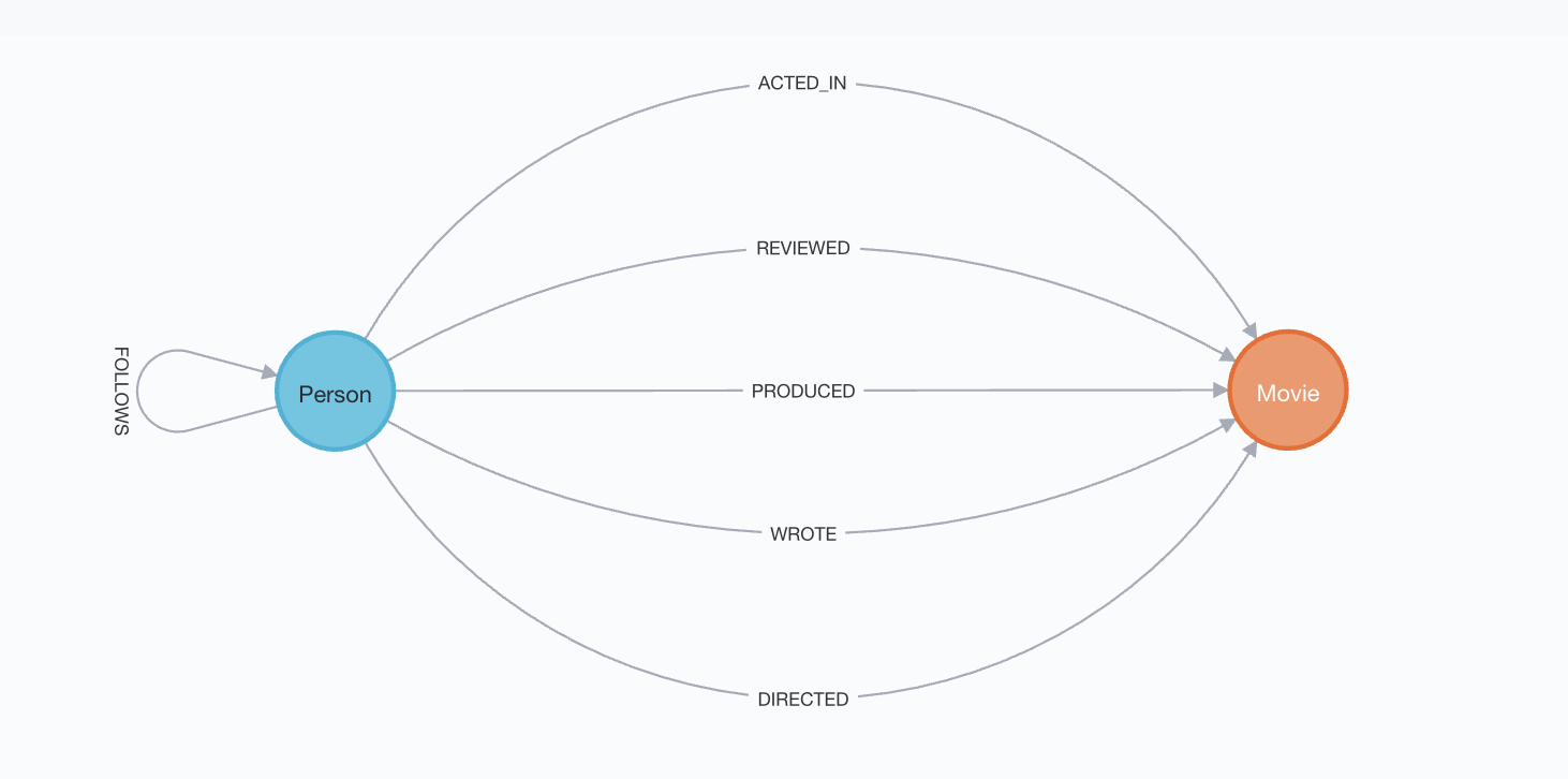
Figure 9.1: Graph schema of the movies database

We can see that there are two types of nodes: Person and Movie. We can also see that a Person can follow another Person, while there are five relationship types between a Person and a Movie. Cypher uses ASCII art to make queries easier to understand and write. Nodes are written in parentheses such as (p:Person) and relationships are written in lines or arrows such as -[:ACTED_IN]->. The following Cypher query will return the graph of all people who acted in movies in the database which were directed by Clint Eastwood, with the results displayed in Figure 9.2.

MATCH (p1:Person)-[:ACTED_IN]->(m:Movie)
MATCH (m:Movie)<-[:DIRECTED]-(p2:Person {name: "Clint Eastwood"})
RETURN p1, m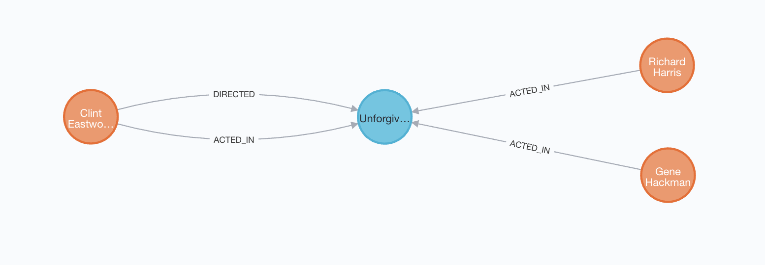

Figure 9.2: Graph of actors in movies directed by Clint Eastwood from movies graph database

Each node or relationship may contain properties which can be accessed and returned in queries. For example, Movie nodes have title and released properties, while Person nodes have a name property. This query will return the actor name, movie title and movie release data, and the result looks like Figure 9.3.

MATCH (p1:Person)-[:ACTED_IN]->(m:Movie)
MATCH (m:Movie)<-[:DIRECTED]-(p2:Person {name: "Clint Eastwood"})
RETURN p1.name AS actor, m.title AS movie, m.released AS released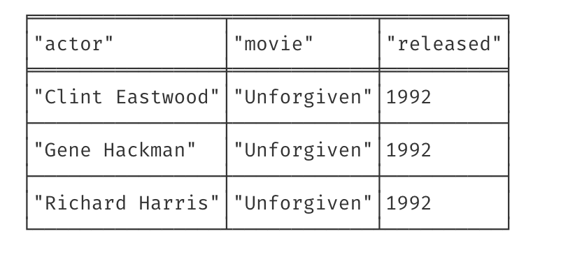

Figure 9.3: Results of a query to find the names of actors, movie title and release date for movies directed by Clint Eastwood in the movies database

Thinking ahead: Neo4J offers a free, sandbox web-based environment through which to learn about its graph database structure and to learn how to write Cypher queries. It includes some interesting graph data sets related to social media analysis, crime investigation, fraud detection, sport and many others. You can start projects in this sandbox and interact with them over the web for a limited period (after which you need to restart a project). You can access the sandbox at https://neo4j.com/sandbox. Later in this chapter, we will go into more detail about working with Neo4J graph databases including how to interact with them in R and in Python, and how to run queries and algorithms against them.

9.1.2 Resource description frameworks

Resource description frameworks (RDFs) are highly flexible graph database models that allow the hierarchical ‘spawning’ of new information in a graph by means of the addition of new nodes. This permits the graph to build more easily organically, because there is no need to worry about whether a given node property already exists in the graph—it can simply be added into a new node that is pointed to by the parent node. For example, imagine that a graph contains nodes that represent people, and imagine that we have some information on the preferred names of those people. Imagine that we have this information for some but not all people, and that some people have a preferred name but others do not. In an RDF, we can create new ‘property edge’ called hasPreferredName which directs to a new node containing the preferred name of the individual.

This high level of flexibility makes RDFs a great choice for ontologies or knowledge graphs for which their development will be unpredictable and will grow organically over time. The low level simplicity of RDFs is the engine behind this flexibility, but this can translate into a complex query language at a high level, making RDFs challenging to deal with for those without specialized knowledge of them. In particular, it can often be necessary to ‘dictate the traversal route’ of the graph in the query language of an RDF, which will require an extensive knowledge of the graph’s structure.

An example of an open, widely used RDF graph is the graph that underlies the Wikipedia online encyclopedia, known as Wikidata⁷⁶. This graph gives structure and connection to the various components of Wikipedia’s content. It helps organize common hierarchical elements of articles and helps link related articles as well as the resources inside those articles such as photos, hyperlinks and so on. As Wikipedia is constantly developing and being added to by a thriving community, this underlying graph needs an extremely high degree of flexibility to support it.

The Wikidata Query Service (WDQS) allows this graph to be queried directly using SPARQL, the standard query language for RDFs. Queries can be submitted at https://query.wikidata.org/, or sent to an API endpoint by an application⁷⁷. Here is an example that will return the top 10 countries of the world in terms of the number of current female city mayors recorded in Wikidata.

SELECT ?countryLabel (count(*) AS ?count)
WHERE
{
    ?city wdt:P31/wdt:P279* wd:Q515 . 
    ?city p:P6 ?hog .           
    ?hog ps:P6 ?mayor .         
    ?mayor wdt:P21 wd:Q6581072 .      
    FILTER NOT EXISTS { ?hog pq:P582 ?x }  
    ?city wdt:P17 ?country .          

    SERVICE wikibase:label {
        bd:serviceParam wikibase:language "en" .
    }
}
GROUP BY ?countryLabel
ORDER BY DESC(?count)
LIMIT 10

Briefly described, the WHERE component of this query instructs a graph traversal as follows:

1. Follow property edges that are ‘instances of cities’ or ‘subclasses of cities’ (call the resulting nodes city)
2. Follow ‘head of government’ property edges from city nodes (call the resulting nodes hog)
3. Follow to retrieve the value of the hog nodes (call this mayor)
4. mayor must have a ‘sex or gender’ property edge that directs to ‘female’
5. Filter results so that hog has no ‘end date’ property edge going from it (that is, current heads of government)
6. Follow ‘country’ property edges from remaining city nodes (call the resulting nodes country)
7. Get the English labels of the country nodes.

This is the core of the query—the remainder simply counts the occurrences of the different country labels and then ranks them in descending order and returns the top 10. You can see how this query requires quite detailed instruction on how to traverse the graph and also needs a very detailed knowledge of a bewildering array of codes for properties and values. RDFs are beautiful and extremely powerful relationship storage engines, but there is a high expertise bar to their use.

Playing around: The query and traversal complexity of RDFs should not be a barrier to you playing around with them. The Wikidata Query Service (WDQS) has a ton of resources to help you understand how to construct interesting queries. For a start, try submitting the above query to WDQS and check the result. If you thought that was fun, some key resources include a long list of example queries⁷⁸ and a Query Builder⁷⁹ which can help non-SPARQL experts to build their own queries.

9.2 Example: how to work with a Neo4J graph database

In this section we will briefly review some ways to work with a Neo4J graph database in order to illustrate how data can be moved into a persistent graph structure for regular query and analysis. First we will look at how to interact with the database via a web browser interface. Then we will look at how to load and query data programmatically via R and Python.

In order to follow the instructions in this section, you will need to set up a free Neo4J Aura graph database. This is a limited instance of a Neo4J graph database hosted on the cloud and offered to developers and learners for free. To do this, follow these steps:

1. Go to the Neo4J Aura site at https://neo4j.com/cloud/aura/ and click ‘Start Free’.
2. Register for free database in a region of your choice and give your database a name.
3. Make a record of your database URI, your username and your password. In the following instructions, we will refer to these as your_URI, your_username and your_password.

In the following examples, we will load our ontariopol data set of the Ontario state politician Twitter network from Chapter 7 into a Neo4J graph database and do some querying against the database.

9.2.1 Using the browser interface

The easiest way to interact with the database is using the browser interface, similar to the Neo4J sandbox mentioned earlier. This is especially useful for beginners who do not need to interact with the database programatically from other applications or data science languages.

Navigate to your free database instance by visiting the Neo4J Aura site, selecting ‘Databases’ from the menu, finding your free database and selecting ‘Open with Neo4J Browser’. After logging in with your credentials, you should be in the browser interface, which looks like Figure 9.4.

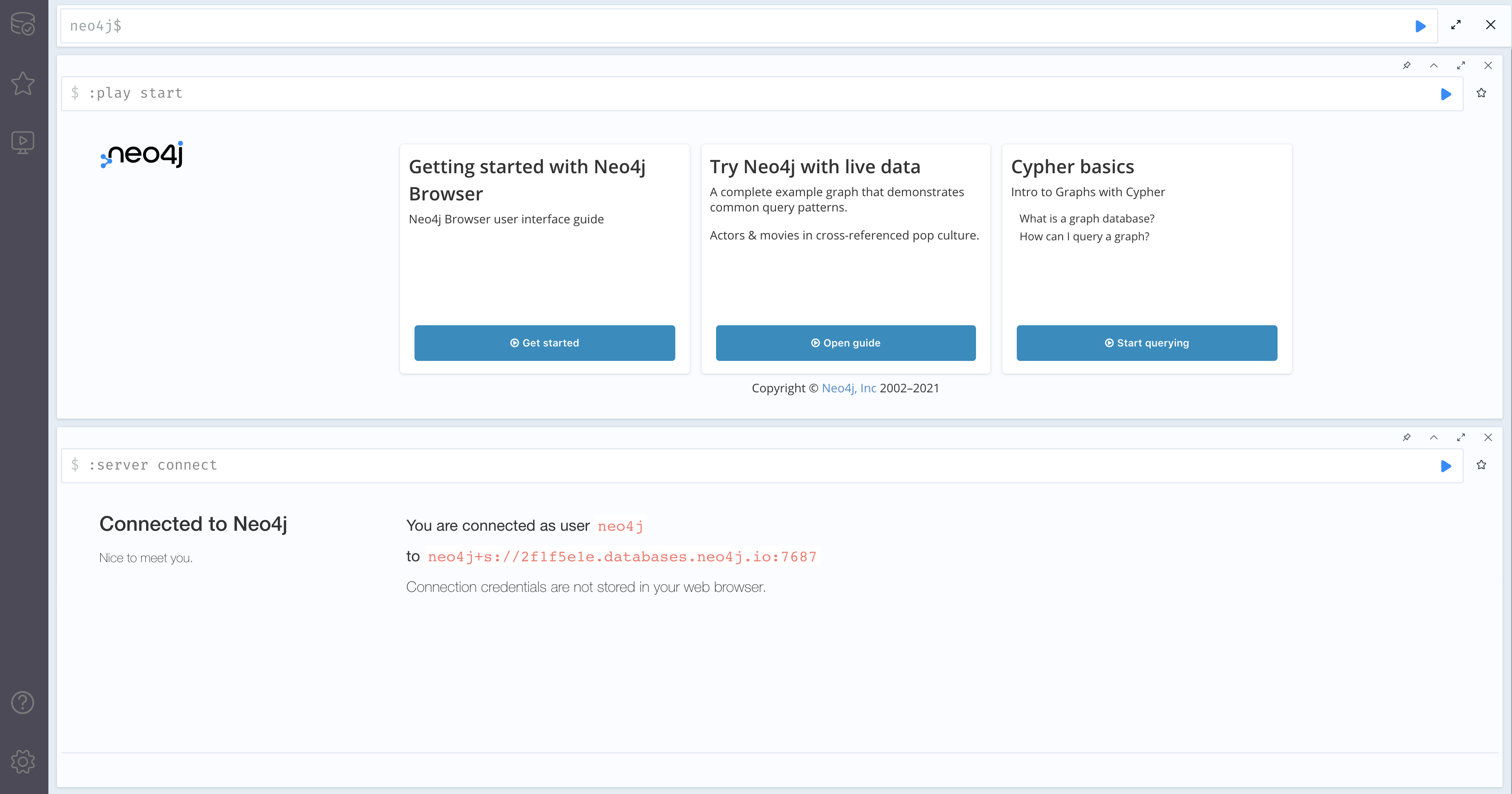
Figure 9.4: The Neo4J browser interface

Cypher queries can be entered in the box at the top⁸⁰. To break a line without submitting the query, press Shift+Enter. To submit the query, press Ctrl+Enter or click the play icon. Before we can start submitting queries, we need to load some data into the database. Among many formats, data can be loaded into Neo4J from an online csv file. Use the following query to load all the vertices from our ontariopol data set.

LOAD CSV WITH HEADERS 
FROM 'https://ona-book.org/data/ontariopol_vertices.csv' 
AS row
MERGE (p:Person {
  personId: row.id, 
  screenName: row.screen_name, 
  name: row.name, 
  party: row.party
});

This query instructs the database to retrieve the data from the specified URL address. It further instructs the database to create nodes called Person nodes from each row of the data. Each Person node should contain four properties: personId, screenName, name and party loaded from the id, screen_name, name and party fields, respectively.

This will load all our Person nodes. You can check that these have been loaded by running this new query:

MATCH (p:Person) 
RETURN p.name;

This query should return the name property of all Person nodes in the graph. Now we need to add the edges using this query:

LOAD CSV WITH HEADERS 
FROM 'https://ona-book.org/data/ontariopol_edgelist.csv' 
AS row
MATCH (p1:Person {personId:row.from}), (p2:Person {personId:row.to})
CREATE (p1)-[:INTERACTED_WITH {weight: toInteger(row.weight)}]-> (p2);

This query instructs the database to load the data from the specified online URL. For each row of the data, it instructs the database to find the Person nodes with personId property corresponding to the from and to fields, to create a directed edge called INTERACTED_WITH between these nodes and to give the edge an integer value weight property extracted from the weight field.

We can now look at our database schema using the following query:

CALL db.schema.visualization();

This should show a very simple schema with one node type and one edge type. By clicking on the database icon in the top left, you should see a further information panel, which should confirm the details of the nodes, the relationships and the properties in the graph, as in Figure 9.5.

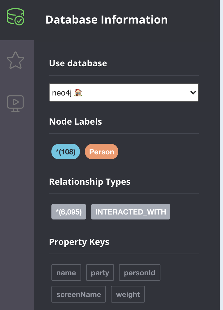
Figure 9.5: The database information panel

Congratulations! You’ve loaded the data into the graph database. Now let’s run a query to find the top 5 politicians who interacted with Christine Elliott based on weight (excluding Christine Elliott herself).

MATCH (p:Person)-[i:INTERACTED_WITH]->({name: "Christine Elliott"})
WHERE p.name <> "Christine Elliott"
RETURN p.name as name, i.weight as weight
ORDER BY weight DESC
LIMIT 5;

This should return a list of 5 with Robin Martin at the top with a weight of 872. As another example, we can try to find out all interactions between LIB party politicians and IND party politicians.

MATCH (p1:Person {party: 'LIB'})-[INTERACTED_WITH]->(p2:Person {party: "IND"})
RETURN p1.name AS LIB_name, p2.name AS IND_name;

This should return 4 interactions. You can also try some procedures from Neo4J’s APOC (Awesome Procedures on Cypher) library. For example, try this to receive information on the distribution of the degrees of the nodes in the graph.

CALL apoc.stats.degrees()

Playing around: Awesome Procedures on Cypher (APOC) is an add-on library which, in its full form, has a very wide range of useful procedures for calculating statistics, finding paths, running search algorithms and much more. As of the time of writing, only a limited number of APOC procedures are available on the free cloud database version we are using here. To see a list of all available APOC procedures, run the query CALL apoc.help('apoc'). If you are interested in the full range of APOC procedures, you can consider installing the Neo4J Desktop product on your local machine for free from the Neo4J website. APOC Full can be installed as an add-on inside the Desktop version, as well as the GDS (Graph Data Science) library, which contains a wide range of graph algorithms including many of the methods we have covered earlier in this book.

9.2.2 Working with Neo4J using R

The neo4jshell package in R allows you to submit queries to a Neo4J database and retrieve results, among other things⁸¹. This package requires the cypher-shell command line utility to be installed on your system. You can install the cypher-shell command line utility standalone by downloading and installing from the Neo4J downloads page⁸². Another option is to download and install the full and free Neo4J community server, which will include cypher-shell, from the community server download page⁸³.

For the neo4j_query() query function to work most smoothly, you should ensure the directory containing the cypher-shell executable is in your system PATH environment variable. Otherwise, you will need to constantly quote the full path to the cypher-shell executable in the shell_path argument of the function.

Assuming you have configured cypher-shell on your system, it is very easy to submit queries to your Neo4J instance and retrieve the results as a dataframe. The first step is to configure your Neo4J connection as a list in R.

neo4j_conn <- list(
  address = "your_URI",
  uid = "your_username",
  pwd = "your_password"
)

In the examples below, we assume that the data has already been loaded to the database using the queries in Section 9.2.1. If not, you can load the data from R by submitting the same queries using the neo4j_query() function. Assuming the data has already been loaded, we can submit a query to the database and retrieve the results as a dataframe. Let’s submit a query to find out the first degree incoming network of all IND party politicians.

# write cypher query
query <- "
MATCH (p:Person)-[:INTERACTED_WITH]->({party: 'IND'})
RETURN DISTINCT p.name AS name, p.party as party;
"

# submit to server and retrieve results as dataframe
results <- neo4jshell::neo4j_query(con = neo4j_conn, qry = query)

# view first few results
head(results)

##                 name party
## 1        Roman Baber   IND
## 2       Deepak Anand   PCP
## 3      Aris Babikian   PCP
## 4       Toby Barrett   PCP
## 5 Peter Bethlenfalvy   PCP
## 6         Will Bouma   PCP

In a similar way we can submit an APOC procedure to obtain statistics about the graph. This query gets statistics on the out-degree of the nodes of the graph.

# get out-degree stats
stats <- neo4jshell::neo4j_query(
  con = neo4j_conn, 
  qry = "CALL apoc.stats.degrees('>');"
)

# extract max, min and mean
stats[c("min", "max", "mean"), ]

## [1] "7"                 "80"                "56.43518518518518"

9.2.3 Working with Neo4J using Python

The py2neo package allows interaction with Neo4J servers from Python. No preconfiguration is required. Connection is established by means of a Graph() object.

import pandas as pd
from py2neo import Graph
import os

# create  connection
neo4j_conn = Graph(
    "your_URI", 
    auth = ("your_username", "your_password")
)

Again, we assume that data has already been loaded to the graph. If this is not the case, submit the data load queries from Section 9.2.1 in the same way as the following examples.

Results from queries will be returned as a list of dicts, which can be converted into the required format.

# write cypher query
query = """
MATCH (p:Person)-[:INTERACTED_WITH]->({party: 'IND'})
RETURN DISTINCT p.name AS name, p.party as party;
"""

# submit to server and retrieve results as list of dicts
results = neo4j_conn.run(query).data()

# convert results to pandas DataFrame and view first few rows
pd.DataFrame(results).head()

##                  name party
## 0         Roman Baber   IND
## 1        Deepak Anand   PCP
## 2       Aris Babikian   PCP
## 3        Toby Barrett   PCP
## 4  Peter Bethlenfalvy   PCP

To run APOC procedures:

# submit APOC procedure
stats = neo4j_conn.run("CALL apoc.stats.degrees('>');").data()

# convert results to pandas DataFrame
pd.DataFrame(stats)

##    type direction  total  p50  p75  p90  p95  p99  p999  max  min       mean
## 0  None  OUTGOING   6095   59   63   70   71   77    80   80    7  56.435185

9.3 Moving to persistent graph data in organizations

The material in this chapter is intended as a brief introduction to the idea of persisting data in a graph database. For organizations that are repeatedly conducting analysis on connections and relationships, this is a natural step to make such analysis more ‘oven ready’. Common transformations which need to be done on data in traditional rectangular databases in order to allow the analysis of connections can be done automatically at regular intervals (weekly, monthly or whatever makes sense based on reporting cadences) and incrementally added to the graph database. An automated ETL (Extract, Transform, Load) process can be set up in R, Python or another platform and timed to run on servers at specified intervals to extract the data from the rectangular databases, perform the necessary transformations to create the data on vertices, edges and properties and then load the data to the graph database.

It should be noted that a graph database is extremely flexible in its ability to store many types of data for many use cases in the same schema. Imagine, for example that we wanted to add the data from our schoolfriends graph to the same graph schema where we loaded the ontariopol data. These are completely different networks, but they can easily coexist in the same graph database. There are many options for how the database could be designed to facilitate this. For example, instead of a single Person node, there could be different Politician and Student nodes. Or we could add a type property to a Person node which could have the value politician or student. Or we could create new Politician and Student nodes and have edges with the relationship IS_A connecting them in a more RDF-like approach.

In all of these cases, the two networks can live in the same database but never interfere with each other, and this model can be scaled arbitrarily as long as it is designed appropriately⁸⁴. This plethora of options means that graph databases often require more up-front schema design consideration compared to traditional databases. Changes in the organization’s data that inevitably occur over time will need to be added to the schema, and some designs will make it more or less easy to do this.

9.4 Learning exercises

9.4.1 Discussion questions

1. Why are graph databases an attractive option for organizations that are regularly performing analysis on connections?
2. Describe labelled-property graphs and resource description frameworks (RDFs). Can you explain some differences between them as graph database technologies, including some pros and cons of their use?
3. Find some examples of real-life use cases of RDFs. Why are RDFs good choices for these use cases?
4. Search some examples of labelled-property graph technologies. What query languages does each use?
5. Describe how Cypher queries are constructed intuitively using ASCII art. Can you find any other query languages that use ASCII art? How similar or different are these languages?

9.4.2 Data exercises

For exercises related to Neo4J, try completing this in the browser and also using either R or Python. Remember that if you are loading data to the graph, be careful to ensure that any previous load of the same data is deleted before reload. If you need to, you can search for help online for Cypher deletion queries, but note that edges must be deleted before nodes.

1. Try to write a SPARQL query and submit it to Wikidata to find the winners of the first ten Eurovision Song Contests. Try a similar query to find the winners of all FIFA World Cups.
2. Write and submit a Cypher query on the ontariopol data loaded to Neo4J to find all interactions from PCP party politicians to LIB party politicians with a weight of greater than 10.
3. Write and submit an APOC procedure on the ontariopol data loaded to Neo4J to obtain the in-degree statistics of the graph.
4. Using the online vertex and edge set for the schoolfriends data set⁸⁵, create a new set of nodes in the Neo4J graph called Student nodes. Give these nodes a name, studentClass and studentGender property from the data sets.
5. Create undirected edges for the Facebook friendships in the data and call the relationship FACEBOOK_FRIENDS. Create directed edges for the reported friendships and call the relationship REPORTED_FRIEND.
6. Write and submit a Cypher query to find all Facebook friends of node 883, and a similar query to find all those who reported node 883 as a friend.
7. Write and submit an APOC procedure to find the node degree statistics for the Facebook friendships. Write and submit separate procedures for the incoming and outgoing reported friendships.