2 Working with Graphs

When we think of a graph, we usually think of a diagram of dots and lines. Indeed, as we have seen in Chapter 1 of this book, the very concept of a graph came into existence in the 1700s when a mathematician tried to solve a problem diagramatically. It makes sense that we think about graphs in this way, because it is intuitive, easy to communicate and in many cases a diagram helps us better address the problem we are solving. However, a diagram is only one way of describing a graph, and it is not particularly scalable. It is easy to draw a diagram for a graph of a few nodes and edges like in our Bridges of Königsberg problem, but what if our problem involved thousands of nodes and millions of edges? Most interesting graphs which we will want to study will be more complex in nature and will contain many hundreds or thousands of nodes and many more edges, and diagrams of graphs of that size are not always useful in helping us solve problems.

In this chapter we will gain a basic understanding of graphs and how to construct them so that we can work with them analytically. We will introduce the most general way of describing a graph mathematically, and we will then discuss how different types of graphs can be defined by placing more conditions on the most general definition. We will go on to look at the different options for how a known graph can be described, including edgelists and adjacency matrices. Equipped with this understanding, we will then learn how to create graph objects in R and in Python. Unlike the larger examples which we will introduce in later chapters, the data and examples we will use in this chapter are simple and straightforward to work with. The focus here is to make sure that the basic structures and definitions are understood before proceeding further. Readers should not skip this chapter if they intend to fully understand the methods and procedures that will be introduced in later chapters.

2.1 Elementary graph theory

The way that graphs are created, stored and manipulated in data science languages like R and Python bears a strong resemblance to how they are defined and studied algebraically. We will start this section with the general mathematical definition of a graph before we proceed to look at different varieties of graphs and different ways of representing graphs using data.

2.1.1 General definition of a graph

A graph \(G\) consists of two sets. The first set \(V\) is known as the vertex set or node set. The second set \(E\) is known as the edge set, and consists of pairs of elements of \(V\). Given that a graph is made up of these two sets, we will often notate our graph as \(G = (V, E)\). If two vertices appear as a pair in \(E\), then those vertices are said to be adjacent or connected vertices.

Let’s use an example to illustrate this definition. Figure 2.1 is a diagram of a graph \(G_{\mathrm{work}}\) with four vertices representing four people. An edge connects two vertices if and only if those two people have worked together.

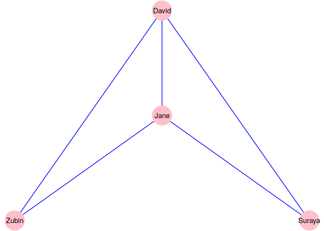
Figure 2.1: A graph \(G_\mathrm{work}\) consisting of four people connected according to whether they have worked together

Our vertex set \(V\) for the graph \(G_{\mathrm{work}}\) is:

\[ V = \{\mathrm{David}, \mathrm{Suraya}, \mathrm{Jane}, \mathrm{Zubin}\} \]

Our edge set \(E\) for the graph \(G_{\mathrm{work}}\) must be notated as pairs of elements of the vertex set \(V\). You can notate this in many ways. One example for how you may notate the edge set is the formal set-theoretic notation:

\[\begin{gather*} E = \{\{\mathrm{David}, \mathrm{Zubin}\}, \{\mathrm{David}, \mathrm{Suraya}\}, \{\mathrm{David}, \mathrm{Jane}\}, \\ \{\mathrm{Jane}, \mathrm{Zubin}\}, \{\mathrm{Jane}, \mathrm{Suraya}\}\} \end{gather*}\]

An alternative notation could also be used such as:

\[\begin{gather*} E = \{\mathrm{David}\longleftrightarrow\mathrm{Zubin}, \mathrm{David}\longleftrightarrow\mathrm{Suraya}, \mathrm{David}\longleftrightarrow\mathrm{Jane}, \\ \mathrm{Jane}\longleftrightarrow\mathrm{Zubin}, \mathrm{Jane}\longleftrightarrow\mathrm{Suraya} \} \end{gather*}\]

It doesn’t really matter how you choose to notate the vertex and edge sets as long as your notation contains all of the information required to construct the graph.

Thinking ahead: If you already know how to load graphs in R or Python, you might want to take a look at a graph object now, and you will see how the object is structured and defined around the two set structure \(G = (V, E)\). For example, try to create a graph from the data for the Bridges of Königsberg problem using the koenigsberg edgelist in the onadata package or downloaded from the internet at https://ona-book.org/data/koenigsberg.csv. Take a look at the vertex set or the edge set to see how they contain the structures discussed here.

The relationship that we are modeling using our edges in the graph \(G_{\mathrm{work}}\) is reciprocal in nature. If David has worked with Zubin, then we automatically conclude that Zubin has worked with David. Therefore, there is no need for direction in the edges of \(G_{\mathrm{work}}\). We call such a graph an undirected graph. In an undirected graph, the order of the nodes in each pair in the edge set \(E\) is not relevant. For example, \(\mathrm{David}\longleftrightarrow\mathrm{Zubin}\) is the same as \(\mathrm{Zubin}\longleftrightarrow\mathrm{David}\).

A graph where direction is important is called a directed graph. As an example, let’s consider a graph \(G_{\mathrm{manage}}\) with the same vertex set of four people but where an edge exists between two people if and only if the first person is the manager of the second person, as in Figure 2.2.

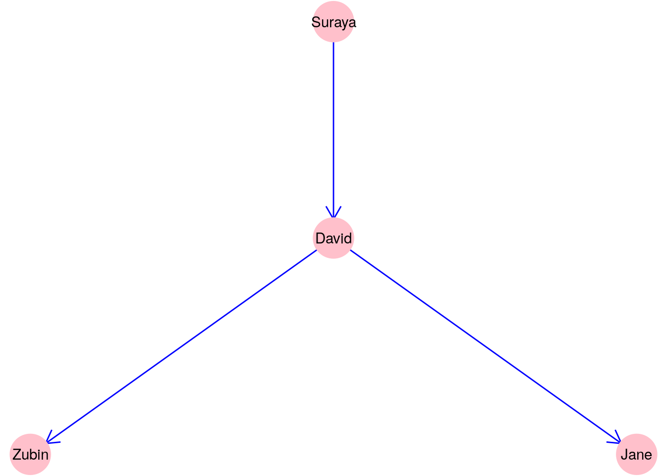
Figure 2.2: A graph \(G_\mathrm{manage}\) consisting of four people connected according to whether one person manages another

Clearly, direction matters in this graph, and therefore we may wish to notate the edge set \(E\) for \(G_{\mathrm{manage}}\) as:

\[ E = \{\mathrm{Suraya}\longrightarrow\mathrm{David}, \mathrm{David}\longrightarrow\mathrm{Zubin}, \mathrm{David}\longrightarrow\mathrm{Jane}\} \]

Note that it is still possible in a directed graph for the edges to point in both directions. While that is unlikely in the case of \(G_{\mathrm{manage}}\) because the manager relationship usually only operates in one direction, imagine another graph \(G_{\mathrm{like}}\) where an edge exists between two people if and only if the first person has listed the second person as someone they like. It is perfectly possible for edges to exist in both directions between two vertices in a graph like this. For example, it may be that Jane likes Zubin and Zubin likes Jane. However, it is important to note that in such a graph, \(\mathrm{Zubin}\longrightarrow\mathrm{Jane}\) and \(\mathrm{Jane}\longrightarrow\mathrm{Zubin}\) are considered two different edges.

Thinking ahead: The graphs \(G_\mathrm{work}\) and \(G_\mathrm{manage}\) are called simple graphs. A simple graph cannot have more than one edge between any two vertices, and cannot have any ‘loop’ edges from one vertex back to itself. As we are about to learn, not all graphs are simple graphs.

2.1.2 Types of graphs

Equipped with our general definition of a graph, we can now define different varieties of graphs by adding or allowing certain conditions on the edges of a general graph. There are many such varieties, but here are a few of the more common graph types.

A multigraph is a graph where multiple edges can occur between the same two vertices. Usually this occurs because the edges are defining different kinds of relationships. Travel routes are common examples of multigraphs, where each edge represents a different carrier. For example, Figure 2.3 is a graph of flights between the San Francisco (SFO), Philadelphia (PHL) and Tucson (TUS) airports based on a data set from December 2010. The graph is layered onto a map of the United States. Philadelphia to Tucson is not a common route and is only offered by one carrier in one direction, while there are multiple carriers operating in both directions between Philadelphia and San Francisco and between San Francisco and Tucson.

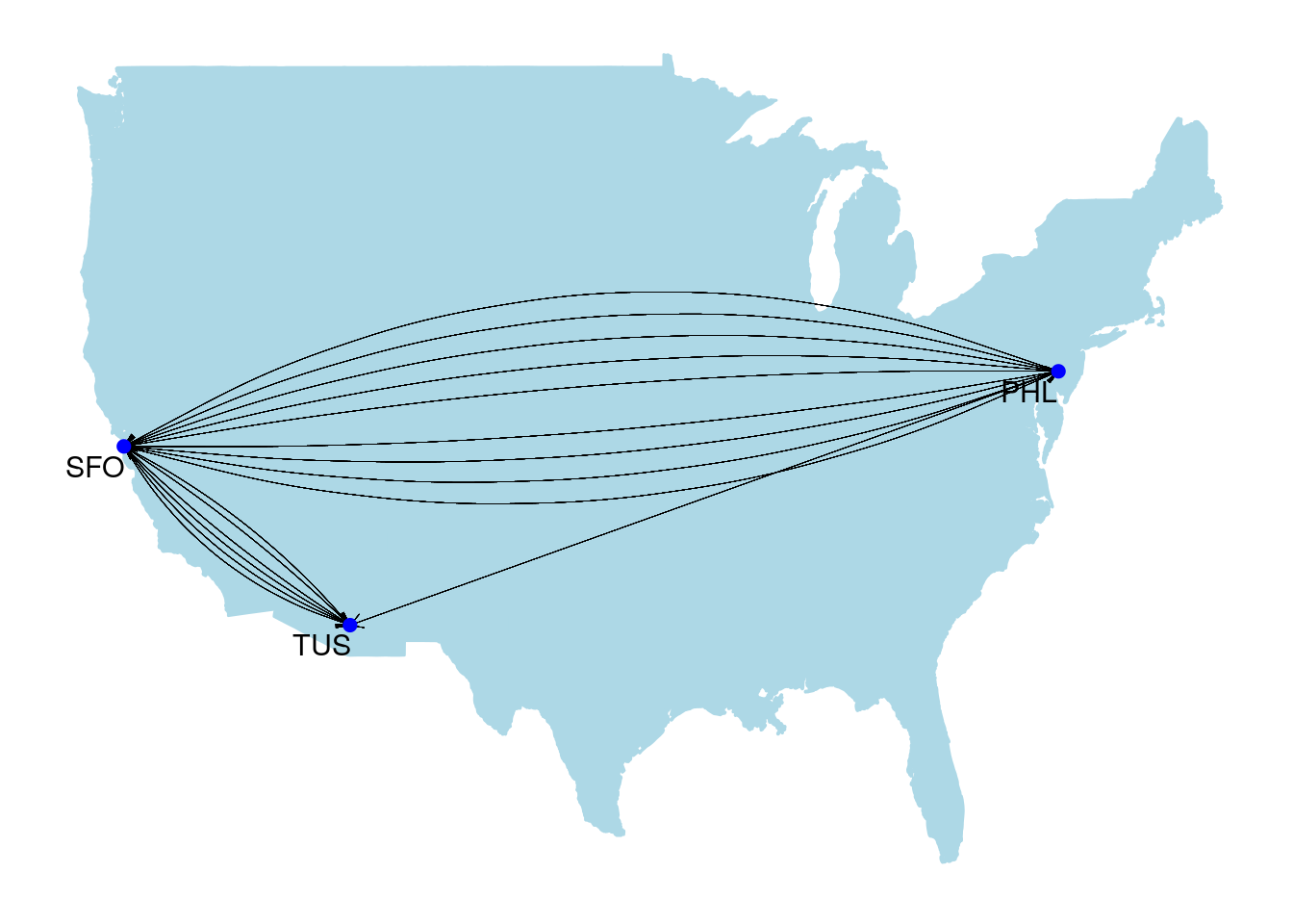
Figure 2.3: Carrier routes operating between three US airports in December 2010

Multigraphs are also commonly used when individuals or entities can be related to each other in different ways. For example, imagine if we were to combine our \(G_{\mathrm{work}}\) and \(G_{\mathrm{manage}}\) graphs from Section 2.1.1 into one single directed graph depicting both ‘worked with’ and ‘manages’ relationships. It might look like Figure 2.4.

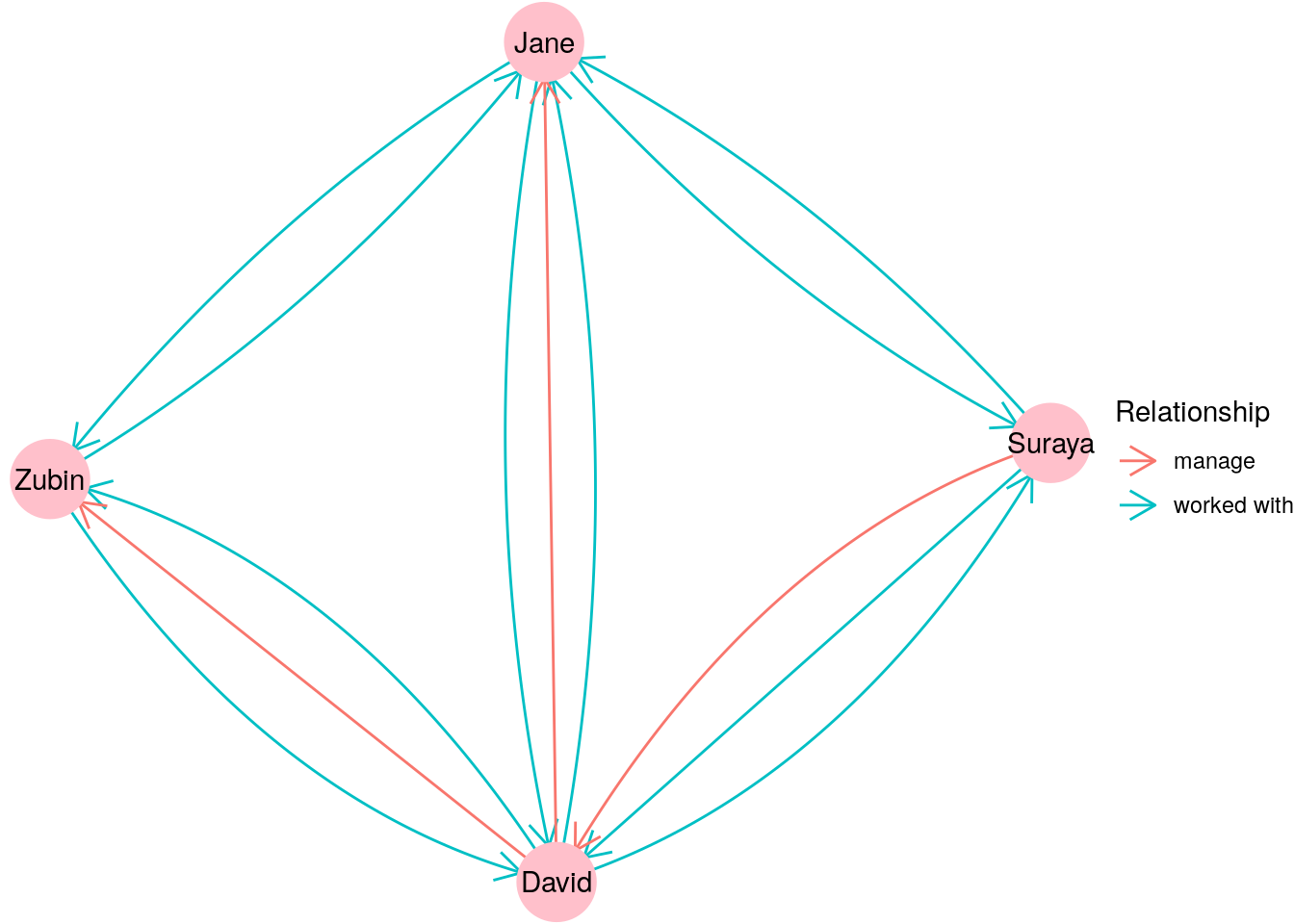
Figure 2.4: Graph depicting different types of relationships between individuals

Many large graphs used in practice are multigraphs, as they are built to capture many different types of relationships between many different types of entities. For example, a graph of an organizational network might contain vertices which represent individuals, organizational units and knowledge areas. Multiple different types of relationships could exist between individuals (such as ‘worked with’, ‘manages’, ‘published with’), between individuals and organizational units (such as ‘member of’ or ‘leader of’), between individuals and knowledge areas (such as ‘affiliated with’ or ‘expert in’) and all sorts of other possibilities.

Pseudographs are graphs which allow vertices to connect to themselves. Pseudographs occur when certain edges depict relationships that can occur between the same vertex. Imagine, for example, a graph \(G_{\mathrm{coffee}}\) which takes our four characters from \(G_{\mathrm{work}}\) in Section 2.1.1 and depicts who buys coffee for whom. If David goes to buy Zubin a coffee, there’s a good chance he will also buy himself one in the process. Thus, you can expect the following edge set:

\[ E = \{\mathrm{David}\longrightarrow\mathrm{Zubin}, \mathrm{David}\longrightarrow\mathrm{David}\} \]

An example of where pseudographs frequently occur might be in the analysis of financial transactions. Let’s imagine that we have a graph of three vertices representing different companies A, B and C, where an edge represents a bank transfer from one company to another on a certain day. If a company holds multiple bank accounts, such a graph might look something like Figure 2.5. An edge which connects a vertex to itself is usually called a loop.

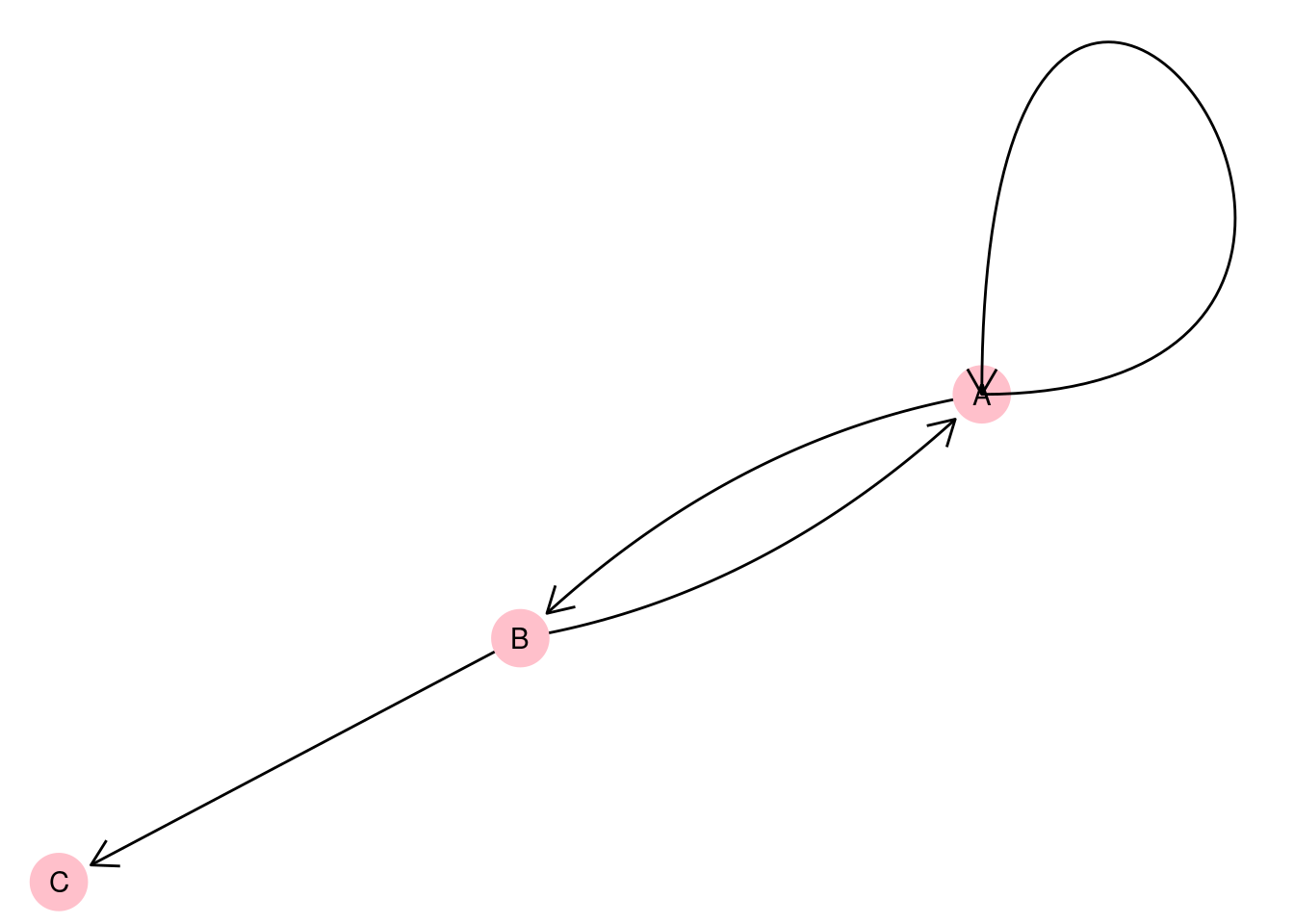
Figure 2.5: Pseudograph representing bank transfers between three companies A, B and C with a loop on vertex A

A complete graph is a graph where all pairs of vertices are connected by an edge. Let’s go back to our four characters in \(G_\mathrm{work}\) from Section 2.1.1. You may notice that only one pair of these characters have not worked together. Let’s assume that we return a month later and update our graph, and it seems that Zubin and Suraya have now worked together. This means our graph becomes a complete graph as depicted in Figure 2.6.

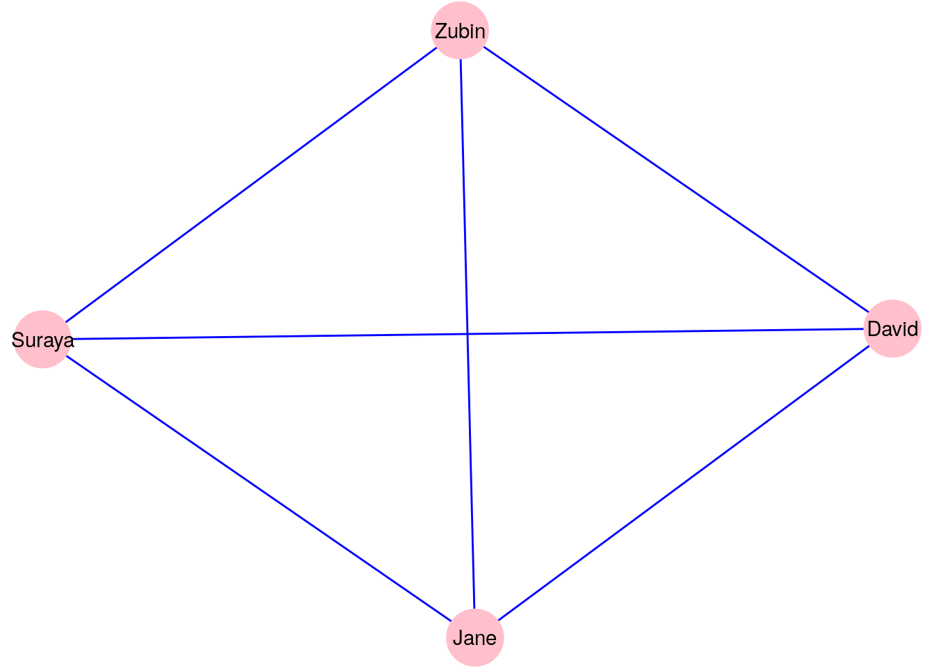
Figure 2.6: Updated version of \(G_\mathrm{work}\) with one additional edge to make it a complete graph

Complete graphs are rare and not very useful in practice, since if you already know that a relationship exists between every pair of vertices, there is not a lot of reason to examine your graph or put it to any practical use. That said, in the field of Graph Theory, it can be important to prove that certain graphs are complete in order to support important theoretical results.

Thinking ahead: While entire graphs which are complete are rarely useful in practice, it is often useful to identify sets of vertices inside graphs which together represent a complete subgraph. Such a group of vertices is known as a clique, and we will look at clique discovery in a later chapter.

Bipartite graphs are graphs that have two disjoint sets of vertices, such that no two vertices in the same set are connected. Imagine we were to add three new individuals from another department to our \(G_\mathrm{work}\) vertices, and redefine our relationships so that an edge means that two individuals worked with each other across departments. Then the new graph \(G_\mathrm{new}\) may look like Figure 2.7, with the distinct sets of vertices representing individuals in different departments.

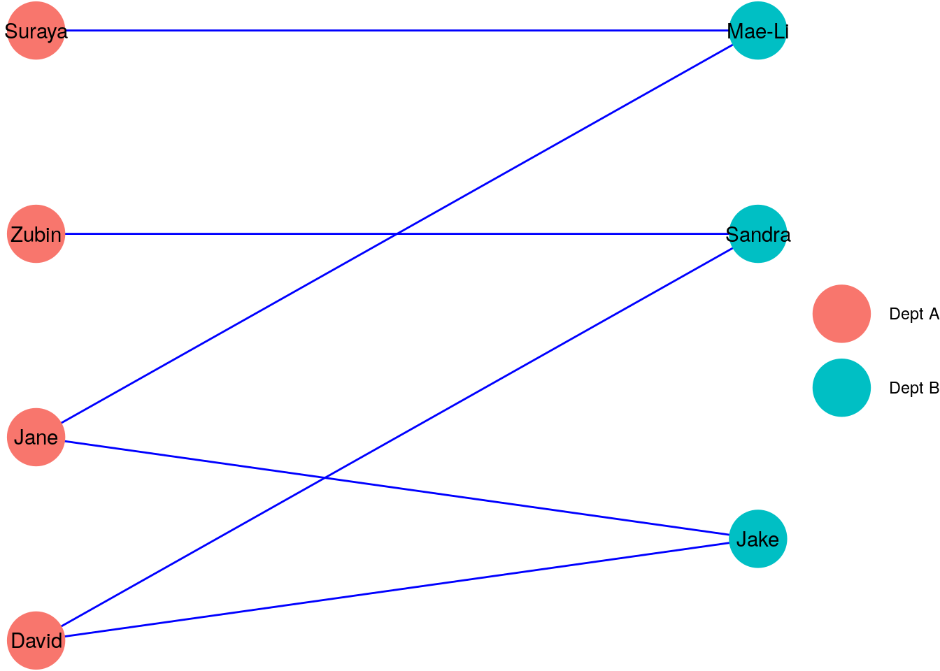
Figure 2.7: A bipartite graph \(G_\mathrm{new}\) showing individuals in different departments A and B working across departments

Extending the idea of bipartite graphs, \(k\)-partite graphs are graphs which have \(k\) disjoint sets of vertices, such that no two vertices in the same set are connected.

Trees can be regarded as vertices connected by edges, and so trees are graphs. For example, our graph \(G_\mathrm{manage}\) in Section 2.1.1 is a tree because it displays a hierarchical management structure between individuals. For a graph to be characterized as a tree, there needs to be exactly one path between any pair of vertices when viewed undirected.

Usually, trees are graphs where the edges represent some sort of hierarchical or nested relationship. Figure 2.8 shows a tree graph of the author’s favorite boy bands, where an edge indicates that the vertex below is a member of the vertex above. It seems like five is the magic number for a great boy band.

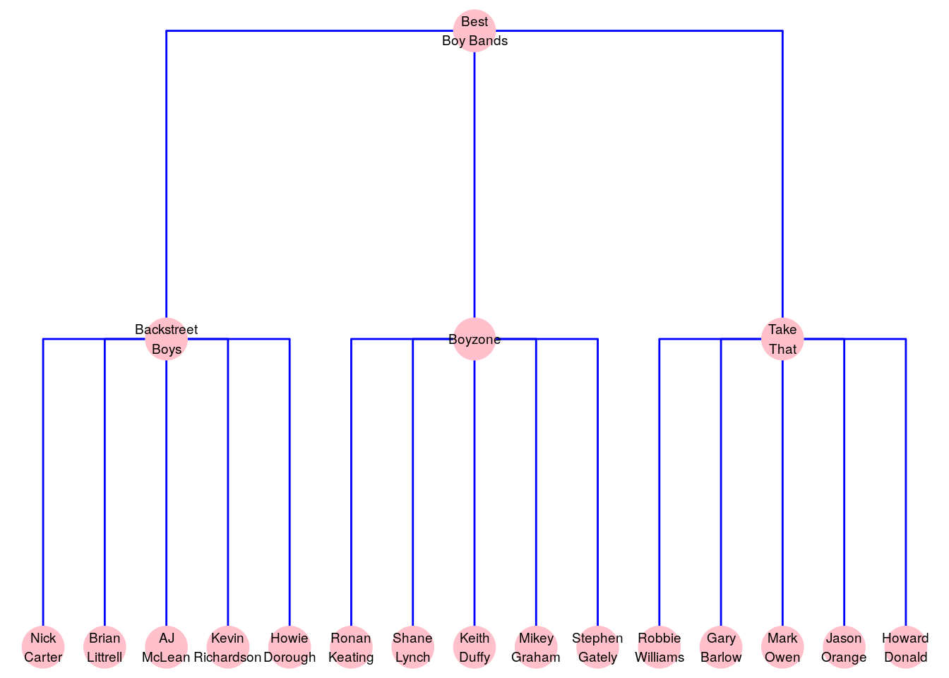
Figure 2.8: Membership of the exclusive class of the author’s favorite boy bands can be represented as a tree graph

2.1.3 Vertex and edge properties

In Section 2.1.1 we learned that a graph \(G = (V, E)\) consists of a vertex set \(V\) and an edge set \(E\). These sets are the minimum elements of a graph—the vertices represent the entities in the graph and the edges represent the relationships between the entities.

We can enhance a graph to provide even richer information on the entities and on the relationships by giving our vertices and edges properties. A vertex property provides more specific information about a vertex and an edge property provides more specific information about the relationship between two vertices.

As an example, let’s return to our directed pseudograph in Figure 2.5, which represents bank transfers between companies A, B, and C. In this graph, we only know from the edges that transfers took place, but we do not know how much money was involved in each transfer, and in what currency the transfer was made. If we wanted to capture this information, we could give each edge properties called amt and cur and store the transfer amount and currency in those edge properties. Similarly, we don’t know a great deal about the companies represented by the vertices. Maybe we would like to know where they are located? If so, we can create a vertex property called loc and store the location in that vertex property.

Figure 2.9 shows this enhanced graph with the vertex and edge properties added diagramatically.

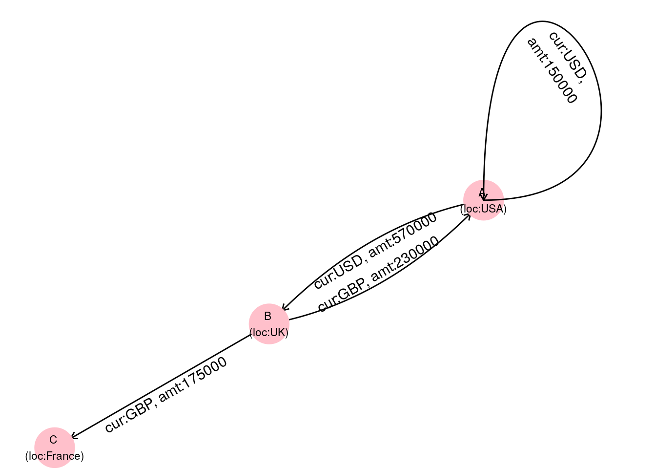
Figure 2.9: Graph of bank transfers between companies A, B and C with additional information stored as vertex and edge properties

Alternatively, we can notate properties as additional sets in our graph, ensuring that each entry is in the same order as the respective vertices or edges, as follows:

\[ \begin{aligned} G &= (V, E, V_\mathrm{loc}, E_\mathrm{cur}, E_\mathrm{amt}) \\ V &= \{A, B, C\} \\ E &= \{A \longrightarrow A, A \longrightarrow B, B \longrightarrow A, B \longrightarrow C\} \\ V_\mathrm{loc} &= \{\mathrm{USA}, \mathrm{UK}, \mathrm{France}\} \\ E_\mathrm{cur} &= \{\mathrm{USD}, \mathrm{USD}, \mathrm{GBP}, \mathrm{GBP}\} \\ E_\mathrm{amt} &= \{150000, 570000, 230000, 175000\} \end{aligned} \]

Note that the vertex property set \(V_\mathrm{loc}\) has the same number of elements as \(V\) and the associated properties appear in the same order as the vertices of \(V\). Note also a similar size and order for the edge property sets \(E_\mathrm{cur}\) and \(E_\mathrm{amt}\). This notation system allows us to provide all the information we need in a reliable way for any number of vertex or edge properties.

Thinking ahead: If you know how to, load up the graph of romantic relationships in the TV Series Mad Men using the madmen_edgelist data set from the onadata package or by downloading it from https://ona-book.org/data/madmen_edgelist.csv. Try to create a graph that contains the Married edge property and then try to query your graph to determine which relationships were marriage relationships.

One of the most common edge properties we will come across is edge weight. Weighted edges are edges which are given a numeric value to represent an important construct such as edge importance or connection strength. This can often be used to simplify otherwise complex graphs, and will be frequently used in calculations related to centrality and community. As an example, returning to our flights graph in Figure 2.3, instead of creating an edge for each carrier, we could simplify our graph by creating one edge per route and giving it a weight according to the number of carriers on that route. Such a graph would look like Figure 2.10.

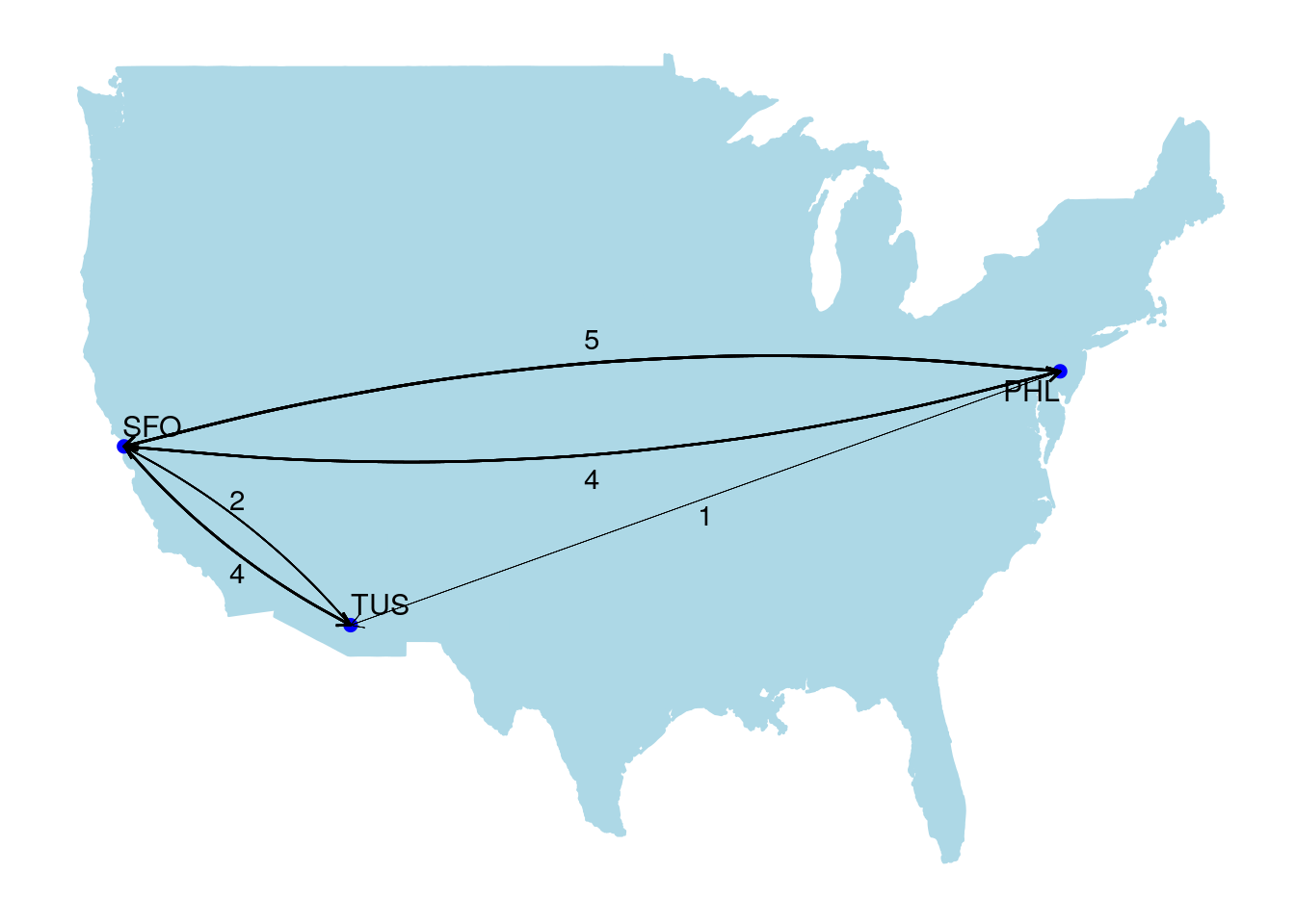
Figure 2.10: Simplifying the flights graph using weighted edges to represent the number of carriers on each route. Edge thickness represents weight.

2.1.4 Representations of graphs

So far in this chapter we have seen two common ways of representing a graph. The first, and most well-known, way is a diagram. The second is an algebraic structure \(G = (V, E)\) consisting (at a minimum) of a vertex set \(V\) and an edge set \(E\). As we discussed at the beginning of this chapter, diagrams are useful for visualizing und understanding small graphs, but less useful for storing graph data and working with large graphs. When working with graphs in the field of data science, the two most common sources of graph data will be edgelists and adjacency matrices.

An edgelist is the edge set \(E\) in our graph \(G = (V, E)\). If we don’t care about isolates¹⁷, then our vertex set \(V\) can be derived directly from \(E\). This means that the edgelist is all that is needed to build a graph provided you are happy to ignore isolates. It is common that an analyst is happy to ignore isolates because we are often only interested in the connections or relationships in the data. Let’s look at an example.

Recall our edge set \(E\) in the graph \(G_\mathrm{work} = (V, E)\) from Section 2.1.1:

\[\begin{gather*} E = \{\mathrm{David}\longleftrightarrow\mathrm{Zubin}, \mathrm{David}\longleftrightarrow\mathrm{Suraya}, \mathrm{Suraya}\longleftrightarrow\mathrm{Jane}, \\ \mathrm{Jane}\longleftrightarrow\mathrm{Zubin}, \mathrm{Jane}\longleftrightarrow\mathrm{Suraya} \} \end{gather*}\]

Since by definition each edge in \(E\) must be a pair of vertices from \(V\), and since we are not concerned about isolates (in fact, we know they don’t exist in this case), we can obtain the vertex set \(V\) by simply listing the unique vertices from the pairs in \(E\). Therefore, we can construct \(V\) to be

\[ V = \{\mathrm{David}, \mathrm{Suraya}, \mathrm{Jane}, \mathrm{Zubin}\} \]

and we now have obtained everything we need for our graph from the edgelist.

Edgelists typically take the form of two columns of data, usually labelled ‘from’ and ‘to’ or ‘source’ and ‘target’. Therefore, our edgelist for \(G_\mathrm{work}\) would look like Table 2.1.

Table 2.1: Edgelist for \(G_\mathrm{work}\)

from	to
David	Zubin
David	Suraya
David	Jane
Jane	Zubin
Jane	Suraya

Playing around: If you still have the Bridges of Königsberg data loaded as a graph in R or Python from earlier, you should be able to generate its edgelist easily. Try to find the right function to use to do this within your package of choice.

An adjacency matrix is a square matrix with the vertices indexing the rows and columns, and where the \((i, j)\)-th entry of the matrix represents the number of edges from vertex \(i\) to vertex \(j\). As an example, using our graph \(G_\mathrm{work}\) again from Section 2.1.1, the adjacency matrix would look like this:

\[ \begin{array}{ccccc} & \mathrm{David} & \mathrm{Jane} & \mathrm{Zubin} & \mathrm{Suraya} \\ \mathrm{David} & 0 & 1 & 1 & 1\\ \mathrm{Jane} & 1 & 0 & 1 & 1 \\ \mathrm{Zubin} & 1 & 1 & 0 & 0 \\ \mathrm{Suraya} & 1 & 1 & 0 & 0 \end{array} \] Adjacency matrices are also commonly written in sparse form, without the use of zeros. For example:

\[ \begin{array}{ccccc} & \mathrm{David} & \mathrm{Jane} & \mathrm{Zubin} & \mathrm{Suraya} \\ \mathrm{David} & . & 1 & 1 & 1\\ \mathrm{Jane} & 1 & . & 1 & 1 \\ \mathrm{Zubin} & 1 & 1 & . & . \\ \mathrm{Suraya} & 1 & 1 & . & . \end{array} \]

An adjacency matrix for an undirected graph like \(G_\mathrm{work}\) is symmetrical on its diagonal, since the existence of an \((i,j)\) edge automatically implies the existence of a \((j, i)\) edge. However, a directed graph may not have a symmetrical adjacency matrix. Here is the adjacency matrix for our \(G_\mathrm{manage}\) graph from Section 2.1.1.

\[ \begin{array}{ccccc} & \mathrm{David} & \mathrm{Jane} & \mathrm{Zubin} & \mathrm{Suraya} \\ \mathrm{David} & . & 1 & 1 & .\\ \mathrm{Jane} & . & . & . & . \\ \mathrm{Zubin} & . & . & . & . \\ \mathrm{Suraya} & 1 & . & . & . \end{array} \]

If a graph is a pseudograph, then the diagonal entries may be greater than zero, and multigraphs can have entries that are any non-negative integer. Here is the adjacency matrix for our flight network graph in Figure 2.3:

\[ \begin{array}{cccc} & \mathrm{SFO} & \mathrm{PHL} & \mathrm{TUS} \\ \mathrm{SFO} & . & 4 & 4 \\ \mathrm{PHL} & 5 & . & 1 \\ \mathrm{TUS} & 2 & . & . \end{array} \]

Thinking ahead: Again, with the Bridges of Königsberg graph loaded in R or Python, you can turn it into an adjacency matrix easily. Try to find the right function for this in your package of choice. Note that in packages like networkx in Python, the format is slightly different and is called an adjacency list.

2.2 Creating graphs in R

In this section we will use some of the examples from the previous section to learn how to create graph objects in R using the igraph package, and to examine the structure of these objects. A strong understanding of how graph objects are structured will make it easier for us to do more advanced manipulation and calculations involving graphs later in the book.

2.2.1 Creating a graph from an edgelist

Let’s start by manually creating an edgelist for our \(G_\mathrm{work}\) graph from Section 2.1.1 as a dataframe in R. We can see this edgelist in Table 2.1. Remember that \(G_\mathrm{work}\) is an undirected graph, so we do not need to worry about edge direction when we create this edgelist.

(gwork_edgelist <- data.frame(
  from = c("David", "David", "David", "Jane", "Jane"),
  to = c("Zubin", "Suraya", "Jane", "Zubin", "Suraya")
))

##    from     to
## 1 David  Zubin
## 2 David Suraya
## 3 David   Jane
## 4  Jane  Zubin
## 5  Jane Suraya

This looks right. Now we are going to load the igraph package and use the function graph_from_edgelist() to create an undirected graph object from this edgelist. This function expects to receive the edgelist as a matrix, and so we will need to convert our gwork_edgelist dataframe to a matrix before we use it in the function.

library(igraph)

gwork_edgelist <- as.matrix(gwork_edgelist)
gwork <- igraph::graph_from_edgelist(el = gwork_edgelist, 
                                     directed = FALSE)

We now have our \(G_\mathrm{work}\) graph in memory. Before we go any further, let’s take a look at it.

gwork

## IGRAPH 7e0127b UN-- 4 5 -- 
## + attr: name (v/c)
## + edges from 7e0127b (vertex names):
## [1] David --Zubin  David --Suraya David --Jane   Zubin --Jane   Suraya--Jane

Let’s start with the string UN-- on the first line of the output. This string describes the type of graph this is. The letter U denotes an undirected graph, and N denotes a graph with named vertices. The two other properties, which we will discover later, are currently not present and so are represented by the dashes --. Next we have the number of vertices (4) and edges (5), followed by two further dashes.

On the next line, the attributes of the graph are listed. In this case there is just one attribute name, which is a vertex attribute of character type—denoted by (v/c). Finally the edges of the graph are given using the vertex names. Note that there is no direction to these edges, so they are denoted with --.

Let’s try the same thing but this time with our directed graph \(G_\mathrm{manage}\) from Section 2.1.1.

gmanage_edgelist <- data.frame(
  from = c("Suraya", "David", "David"),
  to = c("David", "Zubin", "Jane")
)

gmanage_edgelist <- as.matrix(gmanage_edgelist)
(gmanage <- igraph::graph_from_edgelist(el = gmanage_edgelist,
                                       directed = TRUE))

## IGRAPH bfefef5 DN-- 4 3 -- 
## + attr: name (v/c)
## + edges from bfefef5 (vertex names):
## [1] Suraya->David David ->Zubin David ->Jane

We see a similar output to gwork, except we now have a directed graph, donated by D in the first line, and we see that the edges are now denoted with direction using ->.

2.2.2 Creating a graph from an adjacency matrix

Similarly, we can create a graph from data provided in an adjacency matrix. Let’s manually create an adjacency matrix for our flights graph in Figure 2.3, and then we can use the graph_from_adjacency_matrix() function in igraph to create a graph object from the matrix.

# create 3x3 adjacency matrix
adj_flights <- matrix(c(0, 5, 2, 4, 0, 0, 4, 1, 0), nrow = 3, ncol = 3)
rownames(adj_flights) <- c("SFO", "PHL", "TUS")
colnames(adj_flights) <- rownames(adj_flights)

# create multigraph from adjacency matrix
(flightgraph <- igraph::graph_from_adjacency_matrix(
  adjmatrix = adj_flights,
  mode = "directed"
))

## IGRAPH 17d12a7 DN-- 3 16 -- 
## + attr: name (v/c)
## + edges from 17d12a7 (vertex names):
##  [1] SFO->PHL SFO->PHL SFO->PHL SFO->PHL SFO->TUS SFO->TUS SFO->TUS SFO->TUS PHL->SFO PHL->SFO PHL->SFO PHL->SFO
## [13] PHL->SFO PHL->TUS TUS->SFO TUS->SFO

We see the expected directed multigraph with 3 vertices and 16 edges. If we wish to create the weighted graph in Figure 2.10, we add weighted = TRUE to the arguments.

# create weighted graph 
(flightgraph_weighted <- igraph::graph_from_adjacency_matrix(
  adjmatrix = adj_flights,
  mode = "directed",
  weighted = TRUE
))

## IGRAPH 876c006 DNW- 3 5 -- 
## + attr: name (v/c), weight (e/n)
## + edges from 876c006 (vertex names):
## [1] SFO->PHL SFO->TUS PHL->SFO PHL->TUS TUS->SFO

We now see a graph with only 5 edges, but we see the addition of W in our graph type, indicating a weighted graph. We also see a new edge property of numeric type called weight. In situations where we want to simplify multiple edges to single edges without worrying about weight, the simplify() function in igraph works well. By default, simplify() will collapse multiple edges to a single edge and remove any loop edges from vertices to themselves in order to create a simple graph¹⁸.

(flightgraph_simple <- igraph::simplify(
  flightgraph
))

## IGRAPH 62f0716 DN-- 3 5 -- 
## + attr: name (v/c)
## + edges from 62f0716 (vertex names):
## [1] SFO->PHL SFO->TUS PHL->SFO PHL->TUS TUS->SFO

2.2.3 Creating a graph from a dataframe

As we noted in Section 2.1.4, edgelists are usually sufficient to descibe a graph when isolates are not of concern. The function graph_from_edgelist() works fine for this purpose, but it is lacking in flexibility when graphs contain isolates or where vertices have properties that you would ideally like to load on creation. The function graph_from_data_frame() allows you to create a more flexible graph directly from dataframes containing the required data.

Let’s create our bipartite graph \(G_\mathrm{new}\) from Figure 2.7 using this function. At a minimum, this function requires a dataframe of edges, and will also accept a dataframe of vertices if needed.

# edge dataframe
edge_df <- data.frame(
  from = c("David", "David", "Jane", "Jane", "Zubin", "Suraya"),
  to = c("Sandra", "Jake", "Mae-Li", "Jake", "Sandra", "Mae-Li")
) 

# vertex dataframe
vertex_df <- data.frame(
  name = c("David", "Jane", "Zubin", "Suraya", 
           "Sandra", "Jake", "Mae-Li"),
  Dept = c(rep("A", 4), rep("B", 3))
)

# create graph
(gnew <- igraph::graph_from_data_frame(
  d = edge_df,
  directed = FALSE,
  vertices = vertex_df
))

## IGRAPH 945292f UN-- 7 6 -- 
## + attr: name (v/c), Dept (v/c)
## + edges from 945292f (vertex names):
## [1] David --Sandra David --Jake   Jane  --Mae-Li Jane  --Jake   Zubin --Sandra Suraya--Mae-Li

Playing around: The functions in this section are not the only functions in the igraph package that build graphs from data, but they are by far the most commonly used ones. By typing ?graph_from in your R console and looking at the functions that autocomplete, you can see some of the other functions that build graphs from data. Try playing around with them if you are curious.

2.2.4 Adding properties to the vertices and edges

Vertex and edge properties can be added to a new graph at the point of creation or can be added progressively to an existing graph. To add properties at the same time as creating a graph, simply include these properties as columns in the edge or vertex dataframes in the graph_from_data_frame() function. Let’s recreate our financial transaction graph including the edge and vertex properties from Figure 2.9.

# dataframe of edges and properties 
edge_transfers <- data.frame(
  from = c("A", "A", "B", "B"),
  to = c("A", "B", "A", "C"),
  cur = c("USD", "USD", "GBP", "GBP"),
  amt = c(150000, 570000, 230000, 175000)
)

# dataframe of vertices and properties 
vertex_transfers <- data.frame(
  name = c("A", "B", "C"),
  loc = c("USA", "UK", "France")
)

# create graph
(gtransfers <- igraph::graph_from_data_frame(
  d = edge_transfers,
  directed = TRUE,
  vertices = vertex_transfers
))

## IGRAPH c0a0c14 DN-- 3 4 -- 
## + attr: name (v/c), loc (v/c), cur (e/c), amt (e/n)
## + edges from c0a0c14 (vertex names):
## [1] A->A A->B B->A B->C

We see that the additional edge properties cur and amt and the vertex property loc have been included in the graph. The codes immediately following these properties represent the property type and the data type. We can see that loc is a vertex property of character type (v/c), cur is an edge property of character type (e/c) and amt is an edge property of numeric type (e/n).

Playing around: An arbitrary number of properties can be added to the vertices and edges of a graph. If you label one of the properties as weight and if that property is numeric, this will change the type of your graph to W, a weighted graph. Try playing around with this by changing the name of the amt column to weight in gtransfers. Also, earlier we introduced the simplify() function in igraph. The simplify() function helps turn a graph with multiple edges or with loops into a simple graph. However, be careful when using this function if your graph has properties stored in the edges which you need to preserve. Play around with using this function on the gtransfers graph above and see what happens. Experiment with the edge.attr.comb function argument to try to control how the attributes are dealt with when collapsing the edges.

You can view the vertex and edge sets of a graph using the V() and E() functions, respectively.

V(gtransfers)

## + 3/3 vertices, named, from c0a0c14:
## [1] A B C

E(gtransfers)

## + 4/4 edges from c0a0c14 (vertex names):
## [1] A->A A->B B->A B->C

To see specific properties or attributes within the vertices or edges, the $ operator can be used.

V(gtransfers)$name

## [1] "A" "B" "C"

E(gtransfers)$amt

## [1] 150000 570000 230000 175000

Vertex and edge properties can be written into an existing graph directly in this way, providing the properties have the correct length and order. As an example, here is another way of creating our weighted flights graph from Figure 2.10.

# create unweighted graph from routes edgelist
edge_routes <- data.frame(
  from = c("SFO", "SFO", "PHL", "PHL", "TUS"),
  to = c("PHL", "TUS", "SFO", "TUS", "SFO")
) 

edge_routes <- as.matrix(edge_routes)

flightsgraph <- igraph::graph_from_edgelist(
  el = edge_routes,
  directed = TRUE
)

# add weights as an edge property
E(flightsgraph)$weight <- c(4, 4, 5, 1, 2)

# view flightsgraph
flightsgraph

## IGRAPH 1eac512 DNW- 3 5 -- 
## + attr: name (v/c), weight (e/n)
## + edges from 1eac512 (vertex names):
## [1] SFO->PHL SFO->TUS PHL->SFO PHL->TUS TUS->SFO

We see a weighted graph has been created by adding a weight property to the edges of an unweighted graph.

A bipartite graph can be created by giving the vertices a type property according to the two disjoint sets of vertices. Let’s use our \(G_\mathrm{new}\) bipartite graph again as an example, which we generated earlier as the gnew object. In our vertex set, we can define our type property to be the same as the department property Dept.

V(gnew)$type <- V(gnew)$Dept

gnew

## IGRAPH 945292f UN-B 7 6 -- 
## + attr: name (v/c), Dept (v/c), type (v/c)
## + edges from 945292f (vertex names):
## [1] David --Sandra David --Jake   Jane  --Mae-Li Jane  --Jake   Zubin --Sandra Suraya--Mae-Li

We can see that our graph gnew now has the final of the four graph types: B meaning bipartite.

Playing around: Hopefully you can now see that there are many ways to construct your graph. Try using the graph_from_data_frame() function to create gnew as a bipartite graph at the point of creation.

2.3 Creating graphs in Python

In this book we will use the networkx package in Python to create graphs. A version of the igraph package is also available in Python, but networkx contains more convenient functions for building graphs from existing data.

2.3.1 Creating a graph from an edgelist

A graph can be constructed from an edgelist in a Python dictionary. Let’s create our undirected graph \(G_\mathrm{work}\) from Section 2.1.1.

import pandas as pd
import networkx as nx

# create edgelist as dict
gwork_edgelist = dict(
  David = ["Zubin", "Suraya", "Jane"],
  Jane = ["Zubin", "Suraya"]
)

# create graph dict
gwork = nx.Graph(gwork_edgelist)

To view the edges or vertices/nodes, these can be seen as attributes of the gwork object.

# see vertices as list
list(gwork.nodes)

## ['David', 'Jane', 'Zubin', 'Suraya']

# list some edges
list(gwork.edges)[0:3]

## [('David', 'Zubin'), ('David', 'Suraya'), ('David', 'Jane')]

A graph can also be constructed from an edgelist in a Pandas DataFrame. By default, the edgelist needs to have the columns source and target¹⁹.

gwork_edgelist=dict(
  source=["David", "David", "David", "Jane", "Jane"],
  target=["Zubin", "Suraya", "Jane", "Zubin", "Suraya"]
)

#create edgelist as Pandas DataFrame
gwork_edgelist = pd.DataFrame(gwork_edgelist)

# create graph from Pandas DataFrame
gwork = nx.from_pandas_edgelist(gwork_edgelist)

By default these functions use a Graph() class to create an undirected graph. Various methods exist to check the type of graph. For example:

gwork.is_directed()

## False

gwork.is_multigraph()

## False

To create our directed graph \(G_\mathrm{manage}\), we use the DiGraph() class.

gmanage_edgelist=dict(
  David=["Zubin", "Jane"],
  Suraya=["David"]
)

# create directed graph
gmanage=nx.DiGraph(gmanage_edgelist)

# check edges
list(gmanage.edges)

## [('David', 'Zubin'), ('David', 'Jane'), ('Suraya', 'David')]

# check directed
gmanage.is_directed()

## True

2.3.2 Creating a graph from an adjacency matrix

The function from_numpy_matrix() allows the construction of a graph from an adjacency matrix created using numpy. Let’s construct our directed multigraph for flight carriers from Figure 2.3 in this way.

import numpy as np

# create adjacency matrix
adj_flights = np.reshape((0,4,4,5,0,1,2,0,0), (3,3))

# generate directed multigraph 
multiflights = nx.from_numpy_matrix(adj_flights, parallel_edges=True, 
create_using=nx.MultiDiGraph())

# name nodes
label_mapping = {0: "SFO", 1: "PHL", 2: "TUS"}
multiflights = nx.relabel_nodes(multiflights, label_mapping)

# check some edges
list(multiflights.edges)[0:3]

## [('SFO', 'PHL', 0), ('SFO', 'PHL', 1), ('SFO', 'PHL', 2)]

To generate the graph with only single weighted edges as in Figure 2.10, simply change the parallel_edges argument and use the DiGraph() class. This will map the entries in the matrix to a weight edge attribute.

# create with single weighted edges
multiflights = nx.from_numpy_matrix(adj_flights, parallel_edges=False, 
create_using=nx.DiGraph())

# name nodes
label_mapping = {0: "SFO", 1: "PHL", 2: "TUS"}
multiflights = nx.relabel_nodes(multiflights, label_mapping)

# check edges
list(multiflights.edges)

## [('SFO', 'PHL'), ('SFO', 'TUS'), ('PHL', 'SFO'), ('PHL', 'TUS'), ('TUS', 'SFO')]

# check weights of edges
[multiflights.edges[i]['weight'] for i in list(multiflights.edges)]

## [4, 4, 5, 1, 2]

2.3.3 Adding vertex and edge properties to a graph

The easiest way to add attributes to the vertices and edges is to use the set_node_attributes() and set_edge_attributes() functions, respectively. Vertex/node attributes must be passed as a dict with the nodes as keys. Let’s build our financial transactions graph as in Figure 2.9.

# create dict of edgelist
transfer_edgelist = dict(
  A = ["A", "B"],
  B = ["A", "C"]
)

# create directed graph
transfer=nx.DiGraph(transfer_edgelist)

# view vertices
list(transfer.nodes)

## ['A', 'B', 'C']

# add attribute loc to vertices
loc_attributes = dict(A = "USA", B = "UK", C = "France")
nx.set_node_attributes(G = transfer, name = "loc",
values = loc_attributes)

# check 
[transfer.nodes[i]['loc'] for i in list(transfer.nodes)]

## ['USA', 'UK', 'France']

Note that multiple attributes can be set at once by passing a dict of dicts.

# view edges
list(transfer.edges)

## [('A', 'A'), ('A', 'B'), ('B', 'A'), ('B', 'C')]

# add attributes to edges
transfer_attributes = {
  ('A', 'A'): {"cur": "USD", "amt": 150000}, 
  ('A', 'B'): {"cur": "USD", "amt": 570000},
  ('B', 'A'): {"cur": "GBP", "amt": 230000}, 
  ('B', 'C'): {"cur": "GBP", "amt": 175000}
}

# set edge attributes
nx.set_edge_attributes(G = transfer, values = transfer_attributes)

# check
[transfer.edges[i]['cur'] for i in list(transfer.edges)]

## ['USD', 'USD', 'GBP', 'GBP']

[transfer.edges[i]['amt'] for i in list(transfer.edges)]

## [150000, 570000, 230000, 175000]

While this may look tedious and manual, as we move into adding common properties like node centrality or edge weight to graphs, we will find these to be easy to set because of built-in functions that automatically index their output by the vertices or edges. For example, we have already seen in Section 2.3.2 that the function from_numpy_matrix() automatically sets a weight according to the number of edges when we set the argument parallel_edges to False. Also, if you have edge properties as columns in your Pandas edgelist, you can automatically import them into your graph by setting edge_attr = True in the from_pandas_edgelist() function in networkx.

Playing around: As with the igraph package in R, the networkx package in Python contains a whole host of ways to import data into a graph. While the methods outlined here are likely to be the most common, it’s worth taking a look at some of the other functions such as from_dict_of_dicts() or from_dict_of_lists() to see what is available to you.

2.4 Learning exercises

2.4.1 Discussion questions

1. Describe the two sets that make up a graph.
   
2. If a graph has no vertices, then it has no edges. Why is this statement true? Is the converse of this statement true?

For each of the following real-world cases, what kind of graph would be the best choice: a pseudograph, multigraph, \(k\)-partite graph or tree? Also state whether it should be directed or undirected.

3. A graph of academic collaboration where vertices represent people and an edge represents a published paper with both vertices as authors.

4. A graph where each vertex represents a soccer player and an edge exists if both vertices have played on the same team at the same time.

5. A graph where the vertices are geographical cities, countries and continents and an edge exists if one vertex is geographically located in another.

6. A graph where the vertices are a group of colleagues and where an edge exists between vertex \(A\) and vertex \(B\) if at least one email message has been sent from colleague \(A\) to colleague \(B\).

7. A graph where the vertices are world cities grouped by continent, and an edge exists between two cities if an intercontinental flight exists between those cities.

8. What criteria must a graph satisfy to be called a tree?

9. Give two different ways to construct the graph described in Question 3 above.

10. Can you think of three things in your everyday life that could be represented by graphs? What would the vertices and edges represent? What kinds of graph would be best for each case?

2.4.2 Data exercises

Load the koenigsberg edgelist from the onadata package or load it as a dataframe from the internet²⁰. This is the edgelist for the Bridges of Königsberg problem we looked at in Chapter 1. Use your software of choice for the following exercises.

1. Create a graph object using this edgelist. Ensure that it is undirected.
2. By exploring the graph object you just created, determine how many vertices and edges are in this graph. Does this make sense given the original problem tackled by Euler?
3. Obtain a list of the names of the vertices in this graph.
4. Find a function or method in your graph package to create the adjacency matrix or adjacency list for this graph. Check the output to see if it makes sense.

Load the pizza data set from the onadata package or load it as a dataframe from the internet²¹. This data set represents requests made by Reddit users on a thread called Random Acts of Pizza or ROAP, and is part of a larger data set used for research purposes²². The requester column represents users who made requests for pizza, and the responder column represents users who read the request and responded to the request by giving pizza²³. Other columns represent the request ID and data on the requester at the time the request was made.

5. Use an appropriate method to create a graph object using the requester and responder columns in this data set.
6. Use the information contained in the graph object to determine how many pizza requests were fulfilled.
7. Determine using the information in the graph whether anyone fulfilled more than one pizza request.
8. Using an appropriate method, add the other columns in the pizza data set as edge properties.
9. Use the edge properties of your graph object to determine which request ID had the largest number of requester votes.
10. Use the edge properties of your graph object to determine which request ID had the largest number of requester subreddits.