4 Restructuring Data for Use in Graphs
So far we have learned how to define and visualize graphs to allow us to work with them and to gain some basic insights from them. But we have made a really big assumption in doing so. We have assumed that the data we need to create our graph is always available in exactly the form in which we will need it. Usually this is an edgelist or a set of dataframes of edges and vertices. In reality, only certain types of data exist in this form by default. Typically, electronic communication data will often—though not always—have a ‘from’ and ‘to’ structure, because that is how communication works and because many of the underlying systems like email, calendar or other communication networks are already built on databases that have a graph-like structure.
However, there are a lot of problems where we may want to apply graph theory, but where the data does not exist in a way that makes it easy to create a graph. In these situations, we will need to transform the data from its existing shape to a graph-friendly shape—a set of vertices and edges.
There are two important considerations in transforming data into a graph-friendly structure. Both of these considerations depend on the problem you are trying to solve with the graph, as follows:
What entities am I interested in connecting? These will be the vertices of your graph. This could be a single entity type like a set of people, or it could be multiple entity types, such as connecting people to organizational units. Complex graphs will usually involve multiple entity types.
How do I define the relationship between the vertices? These will be the edges of your graph. Again, there can be multiple relationship types, such as ‘reports to’ or ‘works with’, depending on how complex your graph needs to be.
In addition to these fundamental considerations, there are also questions of design in how you construct your graph. This is because there is often more than one option for how you can model the entities and relationships you are interested in. For example, imagine that you have two types of relationships where ‘works with’ means that two people have worked together on the same project and ‘located with’ means that two people are based in the same location. One option for modeling these in a single graph is to have a single entity type (person) connected with edges that have a ‘relationship type’ property (‘works with’ or ‘located with’). Another option is to have several entity types—person, project and location—as vertices, and to connect people to projects and locations using a single edge type that means ‘is a member of’. In the first option, the relationships are modeled directly, but in the second they are modeled indirectly. Both may work equally well for the problem that is being solved by the graph, but one choice may be more useful or efficient than another.
To be able to go about these sorts of transformations requires technical and data design skills and judgment. There is no ‘one size fits all’ solution. The transformations required and how you go about them depends a great deal on the context and the purpose of the work. Nevertheless, in this chapter we will demonstrate two examples which reflect common situations where data needs to be transformed from a graph-unfriendly to a graph-friendly structure. Working through these examples should illustrate a simple design process to follow and help demonstrate typical data transformation methods that could be applied in other common situations.
In the first example, we will study a situation where data exists in traditional rectangular tables, but where we need to transform it in order to understand connections that we cannot understand directly from the tables themselves. This is extremely common in practice and many organizations perform these sorts of transformations in order to populate graph databases from more traditional data sources. In the second example, we will study how to extract information from documents in a way that helps us understand connections between entities in those documents. This is another common situation that has strong applications in general, but has particular potential in the fields of law and crime investigation. Both these examples will be demonstrated in detail using R, and the last section of the chapter will provide examples of how to perform similar transformations using Python.
4.1 Transforming data in rectangular tables for use in graphs
In this example we are going to use some simplified tables from the Chinook database41, an open-source database which contains records of the customers, employees and transactions of a music sales company. We will be working with four simplified tables from this database which you can load from the onadata package now or download from the internet as follows:
# download chinook database tables
chinook_employees <- read.csv(
  "https://ona-book.org/data/chinook_employees.csv"
)
chinook_customers <- read.csv(
  "https://ona-book.org/data/chinook_customers.csv"
)
chinook_invoices <- read.csv(
  "https://ona-book.org/data/chinook_invoices.csv"
)
chinook_items <- read.csv(
  "https://ona-book.org/data/chinook_items.csv"
)
4.1.1 Creating a simple graph of a management hierarchy
First, let’s take a look at a simple example of a graph that already exists explicitly in one of these data tables. Let’s take a look at a few rows of the chinook_employees data set.
##   EmployeeId FirstName LastName ReportsTo
## 1          1    Andrew    Adams        NA
## 2          2     Nancy  Edwards         1
## 3          3      Jane  Peacock         2
## 4          4  Margaret     Park         2
## 5          5     Steve  Johnson         2
## 6          6   Michael Mitchell         1
We can easily create a graph of the management relationships using this table. In such a graph, we would have a single entity type (the employee) as the vertices and the management relationship (‘is a manager of’) as the edges. For simplicity, let’s use first names as vertex names. By joining our data on itself, using EmployeeId = ReportsTo, we can create two columns with the first names of those in each management relationship.
# load dplyr for tidy manipulation in this chapter
library(dplyr)

# create edgelist
(orgchart_edgelist1 <- chinook_employees |>
  dplyr::inner_join(chinook_employees,
                    by = c("EmployeeId" = "ReportsTo")))
## EmployeeId FirstName.x LastName.x ReportsTo EmployeeId.y FirstName.y LastName.y
## 1 1 Andrew Adams NA 2 Nancy Edwards
## 2 1 Andrew Adams NA 6 Michael Mitchell
## 3 2 Nancy Edwards 1 3 Jane Peacock
## 4 2 Nancy Edwards 1 4 Margaret Park
## 5 2 Nancy Edwards 1 5 Steve Johnson
## 6 6 Michael Mitchell 1 7 Robert King
## 7 6 Michael Mitchell 1 8 Laura CallahanWe can see that the FirstName.x column is the manager and so should be the from column and the Firstname.y column should be the to column in our edgelist. We should also remove rows where there is no edge.
(orgchart_edgelist2 <- orgchart_edgelist1 |>
  dplyr::select(from = FirstName.x, to = FirstName.y)) |>
  dplyr::filter(!is.na(from) & !is.na(to))
## from to
## 1 Andrew Nancy
## 2 Andrew Michael
## 3 Nancy Jane
## 4 Nancy Margaret
## 5 Nancy Steve
## 6 Michael Robert
## 7 Michael LauraNow we can create a directed igraph object using the ‘is a manager of’ relationship.
library(igraph)

# create orgchart graph
(orgchart <- igraph::graph_from_data_frame(
  d = orgchart_edgelist2
))
## IGRAPH f6e5835 DN-- 8 7 --
## + attr: name (v/c)
## + edges from f6e5835 (vertex names):
## [1] Andrew ->Nancy Andrew ->Michael Nancy ->Jane Nancy ->Margaret Nancy ->Steve Michael->Robert
## [7] Michael->LauraWe now have a directed graph with named vertices, so this should be easy to plot. Let’s use ggplot with a dendrogram (tree) layout, as in Figure 4.1.
library(ggraph)

# create management structure as dendrogram (tree)
set.seed(123)
ggraph(orgchart, layout = 'dendrogram') +
  geom_edge_elbow() +
  geom_node_label(aes(label = name), fill = "lightblue") +
  theme_void()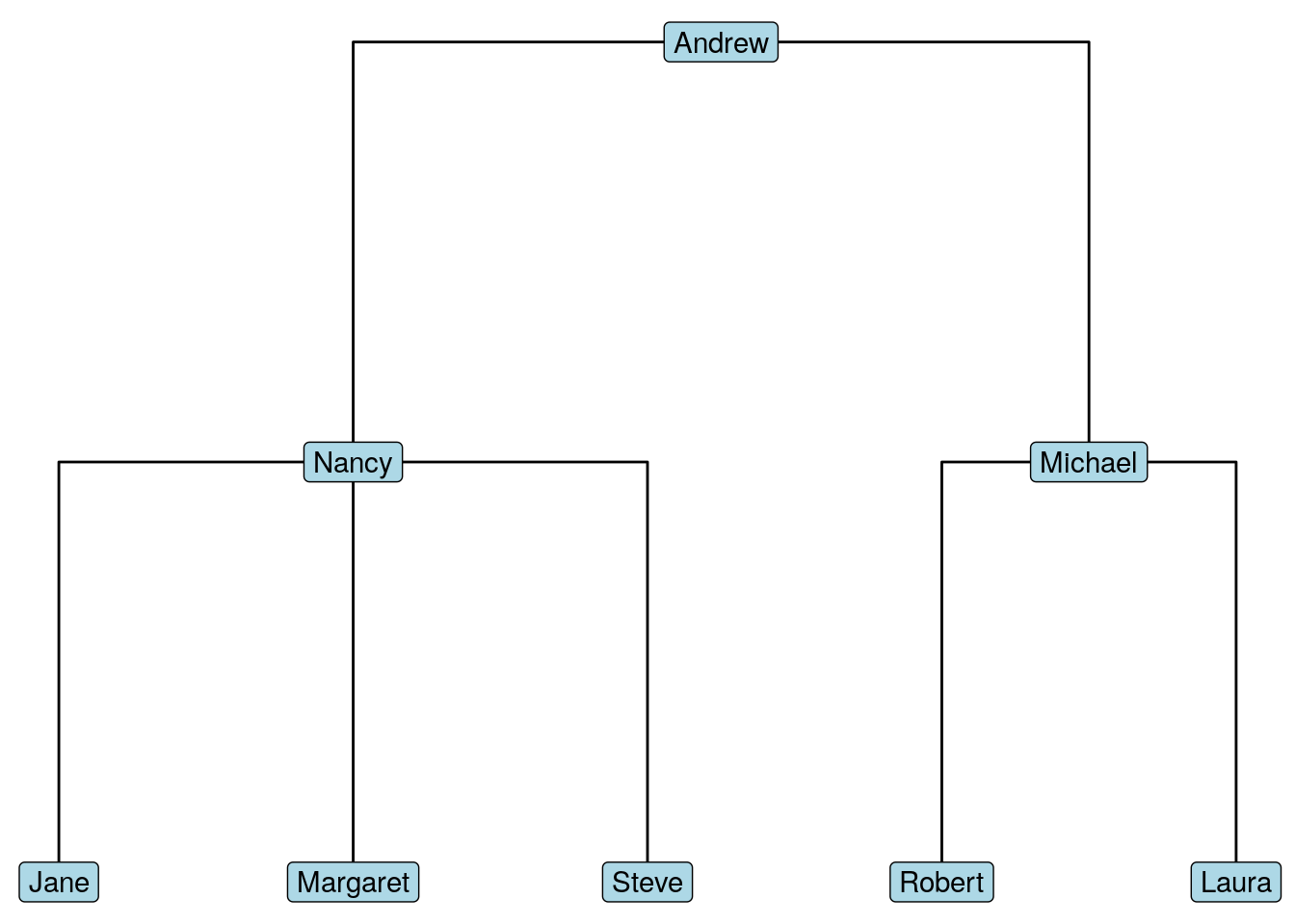
Figure 4.1: Management hierarchy of Chinook as a tree (dendrogram)
4.1.2 Connecting customers through sales reps
Now let’s try to build a graph based an a slightly more complex definition of connection. We are going to connect Chinook’s customers based on whether or not they share the same support rep. First, let’s take a look at the customers table.
##   CustomerId FirstName    LastName SupportRepId
## 1          1      Luís   Gonçalves            3
## 2          2    Leonie      Köhler            5
## 3          3  François    Tremblay            3
## 4          4     Bjørn      Hansen            4
## 5          5 František Wichterlová            4
## 6          6    Helena        Holý            5
We see a SupportRepId field which corresponds to the EmployeeId field in the chinook_employees table. We can join these tables to get an edgelist of customers to support reps. Let’s also create full names for better reference.
# create customer to support rep edgelist
cust_reps <- chinook_customers |>
  dplyr::inner_join(chinook_employees,
                    by = c("SupportRepId" = "EmployeeId")) |>
  dplyr::mutate(
    CustomerName = paste(FirstName.x, LastName.x),
    RepName = paste(FirstName.y, LastName.y)
  ) |>
  dplyr::select(RepName, CustomerName, SupportRepId)

# view head
head(cust_reps)
## RepName CustomerName SupportRepId
## 1 Jane Peacock Luís Gonçalves 3
## 2 Steve Johnson Leonie Köhler 5
## 3 Jane Peacock François Tremblay 3
## 4 Margaret Park Bjørn Hansen 4
## 5 Margaret Park František Wichterlová 4
## 6 Steve Johnson Helena Holý 5Now we have an option of creating two types of graphs. First we could create a graph from the data as is, using the CustomerName and RepName as the edgelist, and where the relationship is ‘is a customer of’. Let’s create that graph, and view it in Figure 4.2. We see a graph with three distinct connected components, each with a hub-and-spoke shape.
# create igraph
cust_rep_graph <- igraph::graph_from_data_frame(
  d = cust_reps
)

# create customer and rep property for vertices
V(cust_rep_graph)$Type <- ifelse(
  V(cust_rep_graph)$name %in% cust_reps$RepName,
  "Rep",
  "Customer"
)

# visualize with color and name aesthetic
set.seed(123)
ggraph(cust_rep_graph, layout = "fr") +
  geom_edge_link(color = "grey", alpha = 0.7) +
  geom_node_label(aes(color = Type, label = name), size = 2) +
  theme_void()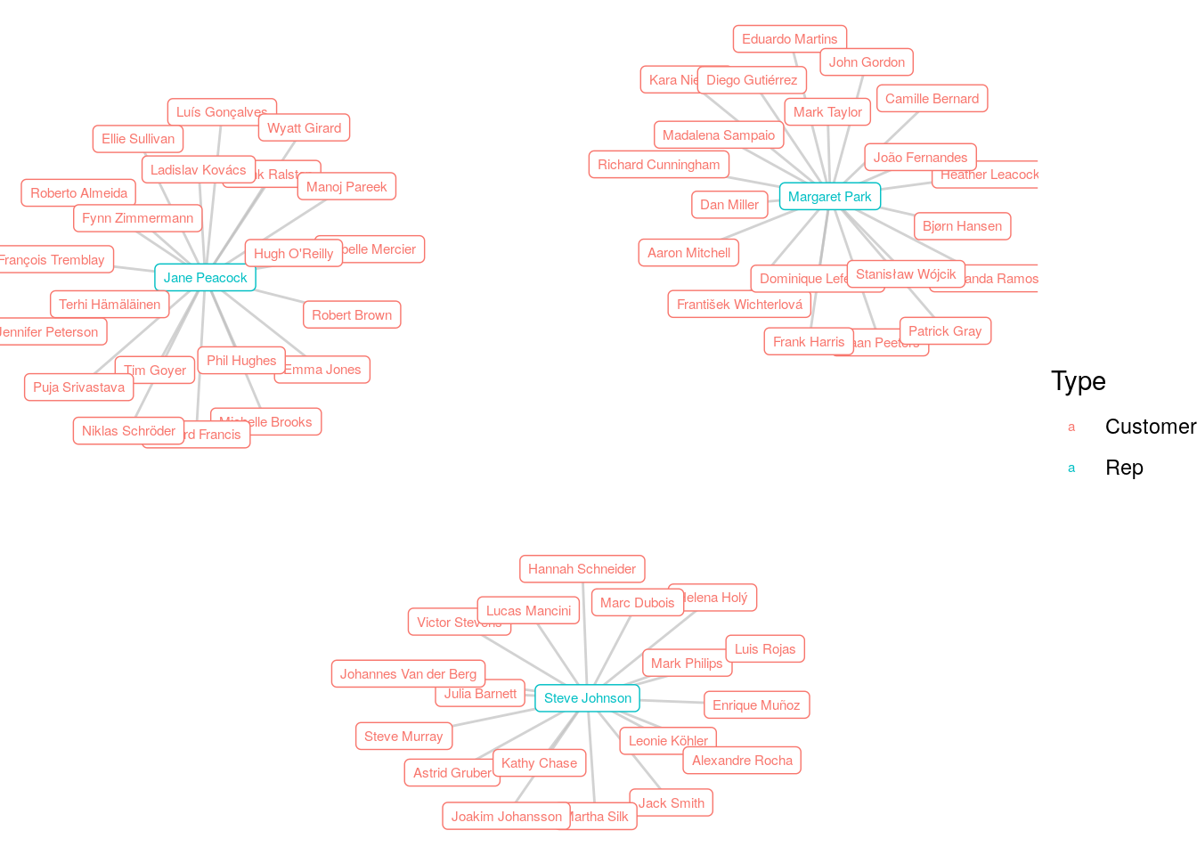
Figure 4.2: Graph of Chinook customers connected to their sales reps
Recall our original objective is to connect customers if they have the same support rep. It is possible to use this graph to do this indirectly, applying the logic that customers are connected if there is a path between them in this graph. However, we may wish to ignore the support reps completely in our graph and make direct connections between customers if they share the same support rep. To do this, we need to do some further joining to our previous cust_reps dataframe.
If we join this dataframe back to our chinook_customers dataframe, we can get customer-to-customer connections via a common support rep as follows:
# connect customers via common support rep
cust_cust <- cust_reps |>
  dplyr::inner_join(chinook_customers, by = "SupportRepId") |>
  dplyr::mutate(Customer1 = CustomerName,
                Customer2 = paste(FirstName, LastName)) |>
  dplyr::select(Customer1, Customer2, RepName)

# view head
head(cust_cust)
## Customer1 Customer2 RepName
## 1 Luís Gonçalves Luís Gonçalves Jane Peacock
## 2 Luís Gonçalves François Tremblay Jane Peacock
## 3 Luís Gonçalves Roberto Almeida Jane Peacock
## 4 Luís Gonçalves Jennifer Peterson Jane Peacock
## 5 Luís Gonçalves Michelle Brooks Jane Peacock
## 6 Luís Gonçalves Tim Goyer Jane PeacockNow we are not interested in creating a pseudograph where customers are connected to themselves, so we should remove any rows where Customer1 and Customer2 are the same.
# remove loop edges
customer_network_edgelist <- cust_cust |>
  dplyr::filter(
    Customer1 != Customer2
  )

# view head
head(customer_network_edgelist)
## Customer1 Customer2 RepName
## 1 Luís Gonçalves François Tremblay Jane Peacock
## 2 Luís Gonçalves Roberto Almeida Jane Peacock
## 3 Luís Gonçalves Jennifer Peterson Jane Peacock
## 4 Luís Gonçalves Michelle Brooks Jane Peacock
## 5 Luís Gonçalves Tim Goyer Jane Peacock
## 6 Luís Gonçalves Frank Ralston Jane PeacockNow we have a network edgelist we can work with, and we have RepName available to use as an edge property. Note that relationships will appear in both directions in this data set, but we can take care of that by choosing to represent them in an undirected graph. Let’s build and visualize the graph, as in Figure 4.3. We see a graph consisting of three complete subgraphs with the edges color coded by the support rep.
# create igraph object
customer_network <- igraph::graph_from_data_frame(
  d = customer_network_edgelist,
  directed = FALSE
)

# visualize
set.seed(123)
ggraph(customer_network) +
  geom_edge_link(aes(color = RepName), alpha = 0.3) +
  geom_node_point(color = "lightblue", size = 6) +
  theme_void()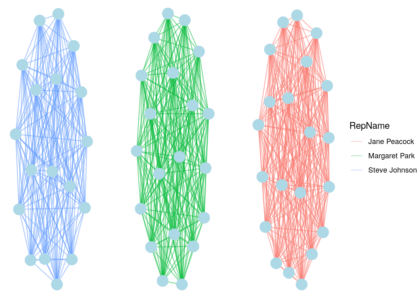
Figure 4.3: Customer-to-customer network for Chinook based on customers sharing the same sales rep
Thinking ahead: Recall from Section 2.1.2 that a complete graph is a graph where every pair of vertices are connected by an edge. Can you see how it follows from the shape of the graph in Figure 4.2 that when we transform the data to produce Figure 4.3, we expect to produce complete subgraphs? Can you also see how visually dense those complete subgraphs are? We will look at the measurement of density in graphs later, but a complete graph will always have a density of 1.
4.1.3 Connecting customers through common purchases
To illustrate a further layer of complexity in reshaping data for use in graphs, let’s imagine that we want to connect customers on the basis of their purchases of common products. We may wish to set some parameters to this relationship; for example, a connection might be based on a minimum number of common products purchased, to give us flexibility around the definition of connection.
To do this we will need to use three tables: chinook_customers, chinook_invoices and chinook_items. To associate a given customer with a purchased item, we will need to join all three of these tables together. Let’s take a quick look at the latter two.
##   InvoiceId CustomerId
## 1         1          2
## 2         2          4
## 3 3 8## InvoiceId TrackId
## 1 1 2
## 2 1 4
## 3 2 6We can regard the TrackId as an item, and using a couple of joins we can quickly match customers with items. It is possible that customers may have purchased the same item numerous times, but we are not interested in that for this work and so we just need the distinct customer and track pairings.
# generate distinct customer-item pairs
cust_item <- chinook_customers |>
  dplyr::inner_join(chinook_invoices) |>
  dplyr::inner_join(chinook_items) |>
  dplyr::mutate(CustName = paste(FirstName, LastName)) |>
  dplyr::select(CustName, TrackId) |>
  dplyr::distinct()

# view head
head(cust_item, 3)
## CustName TrackId
## 1 Luís Gonçalves 3247
## 2 Luís Gonçalves 3248
## 3 Luís Gonçalves 447Similar to our previous example, we can now use this to create an undirected network with two vertex entities: customer and item.
# initiate graph object
customer_item_network <- igraph::graph_from_data_frame(
  d = cust_item,
  directed = FALSE
)

# create vertex type
V(customer_item_network)$Type <- ifelse(
  V(customer_item_network)$name %in% cust_item$TrackId,
  "Item",
  "Customer"
)
This is a big network. Let’s visualize it simply, as in Figure 4.4.
set.seed(123)
ggraph(customer_item_network, layout = "fr") +
  geom_edge_link(color = "grey", alpha = 0.7) +
  geom_node_point(aes(color = Type), size = 2) +
  theme_void()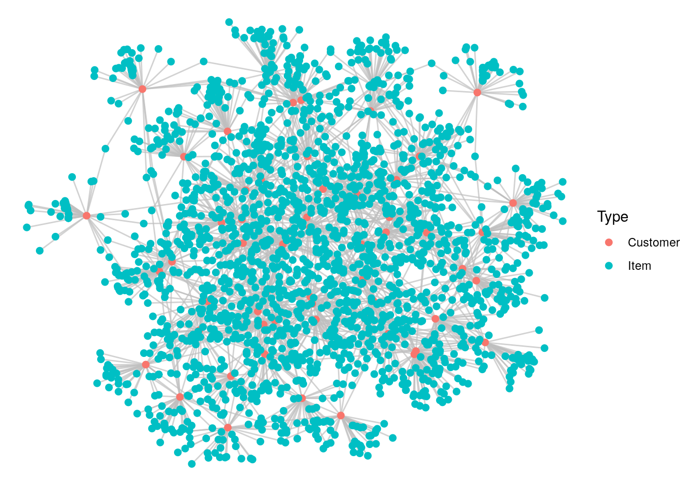
Figure 4.4: Network connecting customers via items purchased
We can see from looking at this graph that there are a large number of items that only one customer has purchased. Therefore, the items themselves seem to be extraneous information for this particular use case. If we are not interested in the items themselves, we can instead create the connections between customers directly. In a similar way to the previous problem, we can join the cust_item table on itself to connect customers based on common item purchases, and we should remove links between the same customer.
# join customers to customers via common items
cust_cust_itemjoin <- cust_item |>
  dplyr::inner_join(cust_item, by = "TrackId") |>
  dplyr::select(CustName1 = CustName.x,
                CustName2 = CustName.y, TrackId) |>
  dplyr::filter(CustName1 != CustName2)

# view head
head(cust_cust_itemjoin)
## CustName1 CustName2 TrackId
## 1 Luís Gonçalves Edward Francis 449
## 2 Luís Gonçalves Richard Cunningham 1157
## 3 Luís Gonçalves Richard Cunningham 1169
## 4 Luís Gonçalves Astrid Gruber 2991
## 5 Luís Gonçalves Emma Jones 280
## 6 Luís Gonçalves Emma Jones 298The issue with this data set is that it will count every instance of a common item purchase twice, with the customers in opposite orders, and this is double counting. So, we need to group the pairs of customers irrelevant of their order and ensure we don’t double up on items.
# avoid double counting
cust_item_network <- cust_cust_itemjoin |>
  dplyr::group_by(Cust1 = pmin(CustName1, CustName2),
                  Cust2 = pmax(CustName1, CustName2)) |>
  dplyr::summarise(TrackId = unique(TrackId), .groups = 'drop')

# view head
head(cust_item_network)
## # A tibble: 6 × 3
## Cust1 Cust2 TrackId
## <chr> <chr> <int>
## 1 Aaron Mitchell Alexandre Rocha 2054
## 2 Aaron Mitchell Bjørn Hansen 1626
## 3 Aaron Mitchell Enrique Muñoz 2027
## 4 Aaron Mitchell Hugh O'Reilly 2018
## 5 Aaron Mitchell Niklas Schröder 857
## 6 Aaron Mitchell Phil Hughes 1822If that worked, we should see that the table cust_cust_itemjoin has twice as many rows as cust_item_network.
## [1] 2This looks good. So we now can count up how many common items each pair of customers purchased.
# count common items
cust_item_network <- cust_item_network |>
  dplyr::count(Cust1, Cust2, name = "Items")

# view head
head(cust_item_network)
## # A tibble: 6 × 3
## Cust1 Cust2 Items
## <chr> <chr> <int>
## 1 Aaron Mitchell Alexandre Rocha 1
## 2 Aaron Mitchell Bjørn Hansen 1
## 3 Aaron Mitchell Enrique Muñoz 1
## 4 Aaron Mitchell Hugh O'Reilly 1
## 5 Aaron Mitchell Niklas Schröder 1
## 6 Aaron Mitchell Phil Hughes 1We are now ready to construct our customer-to-customer graph, with Items as an edge property. We can visualize it with an edge color code indicating how many common items were purchased, as in Figure 4.5.
# create undirected graph
custtocust_network <- igraph::graph_from_data_frame(
  d = cust_item_network,
  directed = FALSE
)

# visualize with edges color coded by no of items
set.seed(123)
ggraph(custtocust_network) +
  geom_edge_link(aes(color = ordered(Items)), alpha = 0.5) +
  geom_node_point(color = "lightblue", size = 6) +
  labs(edge_color = "# of Common Items") +
  theme_void()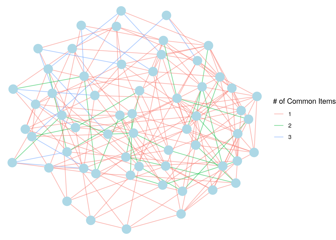
Figure 4.5: Chinook customer-to-customer network based on common item purchases
If we wish, we can restrict the definition of connection. For example, we may define it as ‘purchased at least two items in common’, as in Figure 4.6. We can use the subgraph() function in igraph for this, and the result reveals a graph with two connected components, indicating that there are two independent groups of customers who are related according to some commonality in music purchasing.
# select edges that have Item value of at least 2
edges <- E(custtocust_network)[E(custtocust_network)$Items >= 2]

# create subgraph using these edges
two_item_graph <- igraph::subgraph.edges(custtocust_network,
                                         eids = edges)

# visualise
set.seed(123)
ggraph(two_item_graph, layout = "fr") +
  geom_edge_link(color = "grey", alpha = 0.7) +
  geom_node_point(color = "lightblue", size = 6) +
  theme_void()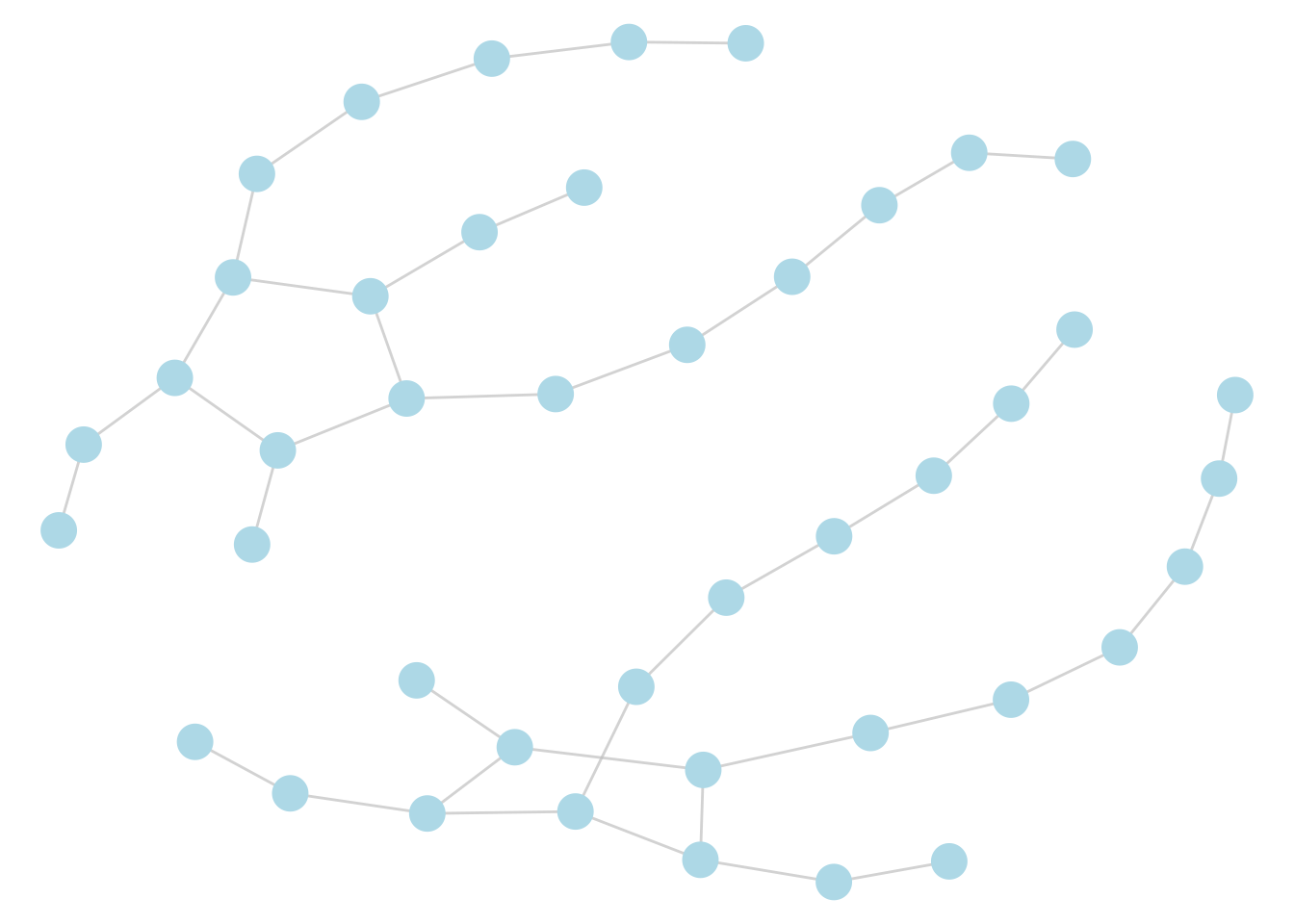
Figure 4.6: Chinook customer-to-customer network based on at least two common items purchased
4.1.4 Approaches using Python
To illustrate similar approaches in Python, we will redo the work in Section 4.1.3. First, we will download the various data sets.
import pandas as pd
import numpy as np

# download chinook database tables
chinook_customers = pd.read_csv(
  "https://ona-book.org/data/chinook_customers.csv"
)
chinook_invoices = pd.read_csv(
  "https://ona-book.org/data/chinook_invoices.csv"
)
chinook_items = pd.read_csv(
  "https://ona-book.org/data/chinook_items.csv"
)
Now we join the three tables together, create the FullName variable and ensure that we don’t have any duplicate relationships:
# join customers to invoices
joined_tables = pd.merge(
  chinook_customers,
  chinook_invoices
)

# join result to items
joined_tables = pd.merge(joined_tables, chinook_items)

# create FullName
joined_tables['FullName'] = joined_tables['FirstName'] + ' ' + \
joined_tables['LastName']

# drop duplicates and view head
cust_item_table = joined_tables[['FullName', 'TrackId']]\
.drop_duplicates()
cust_item_table.head()
## FullName TrackId
## 0 Luís Gonçalves 3247
## 1 Luís Gonçalves 3248
## 2 Luís Gonçalves 447
## 3 Luís Gonçalves 449
## 4 Luís Gonçalves 451Now we can create a graph of connections between customers and items and visualize it as in Figure 4.7.
import networkx as nx
from matplotlib import pyplot as plt

# create networkx object
cust_item_network = nx.from_pandas_edgelist(cust_item_table,
source = "FullName", target = "TrackId")

# color items differently to customers
colors = ["red" if i in cust_item_table['FullName'].values else "green"
for i in cust_item_network.nodes]

# visualize
np.random.seed(123)
nx.draw_networkx(cust_item_network, node_color = colors, node_size = 2,
edge_color = "grey", with_labels = False)
plt.show()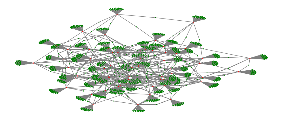
Figure 4.7: Visualization of the Chinook customer-to-item network with customers as red vertices and items as green vertices
Now to create the customer-to-customer network based on common item purchases, we do further joins on the data sets and remove connections between the same customers.
# merge customers on common track IDs
cust_cust_table = pd.merge(cust_item_table, cust_item_table,
on = "TrackId")

# rename columns
cust_cust_table.rename(
  columns={'FullName_x' :'CustName1', 'FullName_y' :'CustName2'},
  inplace=True
)

# remove loop edges
cust_cust_table = cust_cust_table[
  ~(cust_cust_table['CustName1'] == cust_cust_table['CustName2'])
]

# view head
cust_cust_table.head()
## CustName1 TrackId CustName2
## 4 Luís Gonçalves 449 Edward Francis
## 5 Edward Francis 449 Luís Gonçalves
## 11 Luís Gonçalves 1157 Richard Cunningham
## 12 Richard Cunningham 1157 Luís Gonçalves
## 17 Luís Gonçalves 1169 Richard CunninghamNow we can drop duplicates based on the TrackId, count the items by pair of customers, and we will have our final edgelist:
# drop duplicates
cust_cust_table = cust_cust_table.drop_duplicates('TrackId')

# count common items
cust_cust_table = cust_cust_table.groupby(['CustName1', 'CustName2'],
as_index = False).TrackId.nunique()
cust_cust_table.rename(columns = {'TrackId': 'Items'}, inplace = True)

# view head
cust_cust_table.head()
## CustName1 CustName2 Items
## 0 Aaron Mitchell Enrique Muñoz 1
## 1 Aaron Mitchell Hugh O'Reilly 1
## 2 Aaron Mitchell Niklas Schröder 1
## 3 Aaron Mitchell Phil Hughes 1
## 4 Alexandre Rocha Aaron Mitchell 1Now we are ready to create and visualize our customer-to-customer network, as in Figure 4.8.
# create networkx object
cust_cust_network = nx.from_pandas_edgelist(cust_cust_table,
source = "CustName1", target = "CustName2", edge_attr = True)


# visualize
np.random.seed(123)
nx.draw_networkx(cust_cust_network, node_color = "lightblue",
edge_color = "grey", with_labels = False)
plt.show()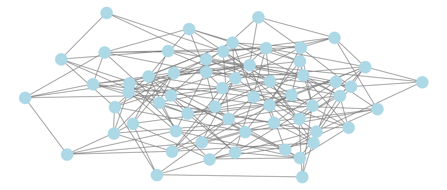
Figure 4.8: Visualization of the Chinook customer-to-customer network based on any common item purchase
And if we wish to restrict connections to two or more common item purchases, we can create a subgraph based on the number of items, as in Figure 4.9. Some experimentation with the parameter k in networkx’s spring layout (which determines the optimal distance between vertices) is needed to appropriately visualize the two distinct connected components in this graph.
# get edges with items >= 2
twoitem_edges = [i for i in list(cust_cust_network.edges) if
cust_cust_network.edges[i]['Items'] >= 2]

# create subgraph
twoitem_network = cust_cust_network.edge_subgraph(twoitem_edges)

# visualize in FR (spring) layout
np.random.seed(123)
layout = nx.spring_layout(twoitem_network, k = 0.05)
nx.draw_networkx(twoitem_network, node_color = "lightblue",
edge_color = "grey", with_labels = False, pos = layout)
plt.show()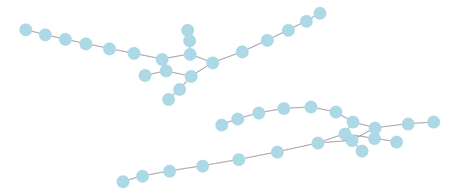
Figure 4.9: Visualization of the Chinook customer-to-customer network based on at least two common item purchases
4.2 Transforming data from documents for use in graphs
In our second example, we will look at how to extract information that sits in semi-structured documents and how to convert that information to a graph-like shape to allow us to understand relationships that interest us. Semi-structured documents are documents which have a certain expected format through which we can reliably identify important actors or entities. These could be legal contracts, financial statements or other types of structured forms. Through extracting entities from these documents, we can identify important relationships between them, such as co-publishing, financial transactions or contractual obligations.
To illustrate this, we will show how to extract information from a TV script in a way where we can determine which characters have spoken in the same scene together, and then use this information to create a network of TV characters. We will use an episode script from the hit TV comedy show Friends. A full set of scripts from all episodes of Friends can be found online at https://fangj.github.io/friends/. For this learning example, we will focus on the character network from the first episode of Friends. The script of the first episode can be found at https://fangj.github.io/friends/season/0101.html. Once we have learned the basic methods using the first episode, some of the end-of-chapter exercises will encourage the extension of these methods to further episodes.
4.2.1 Scraping data from semi-structured documents
First, we will look at how to obtain a list of numbered scenes and the characters in each scene, through ‘scraping’ these details from the online script. To help us with this, we will use the rvest R package, which is designed for scraping information from webpages.
Let’s take a look at the web code for Season 1, Episode 1. You can do this by opening the script webpage in Google Chrome and then pressing Cmd+Option+C (or Ctrl+Shift+C in Windows) to open the Elements Console where you can view the HTML code of the page side-by-side with the page itself. This should look like Figure 4.10.
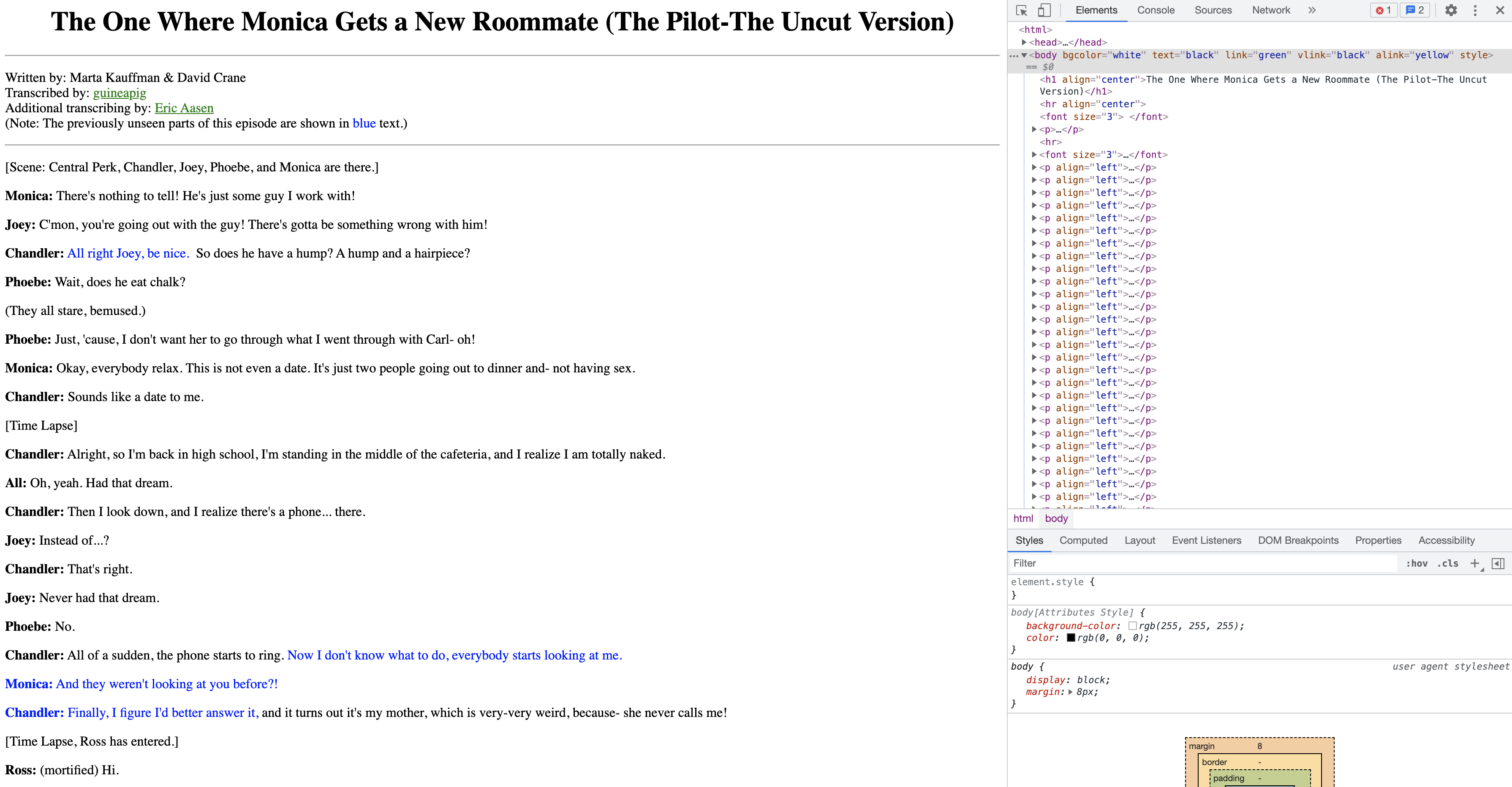
Figure 4.10: Viewing the script of Season 1, Episode 1 of Friends with the Elements console open in Google Chrome
One of the things we can see immediately is that most of the words that precede a colon are of interest to us. In fact, most of them are character names that say something in a scene. We also see that lines that contain the string “Scene:” are pretty reliable indicators of scene boundaries.
The first thing we should do is get this HTML code in a list or vector of HTML nodes which represent the different pieces of formatting and text in the document. Since this will contain the separated lines spoken by each character, this will be really helpful for us to work from. So let’s download the HTML code and break it into HTML nodes so that we have a nice, tidy vector of script content.
# loading rvest also loads the xml2 package
library(rvest)

url_string <- "https://fangj.github.io/friends/season/0101.html"

# get script as vector of HTML nodes
nodes <- xml2::read_html(url_string) %>%
      xml2::as_list() %>%
      unlist()

# view head
head(nodes)
## html.head.title
## "The One Where Monica Gets a New Roomate (The Pilot-The Uncut Version)"
## html.body1
## "\n\n"
## html.body.h1
## "The One Where Monica Gets a New Roommate (The Pilot-The Uncut Version)"
## html.body3
## "\n\n"
## html.body.font
## "\n\n"
## html.body.font.p
## "Written by: Marta Kauffman & David Crane"This has generated a named character vector that contains a lot of different splitout parts of the script, but most importantly it contains the lines from the script, for example:
##                                                       html.body.font.p
## "[Scene: Central Perk, Chandler, Joey, Phoebe, and Monica are there.]"
Now, to generate something useful for our task, we need to create a vector that contains the word ‘New Scene’ if the line represents the beginning of a scene, and the name of the character if the line represents something spoken by a character. This will be the best format for what we want to do.
The first thing we will need to do is swap any text string containing “Scene:” to the string “New Scene”. We can do this quite simply using an ifelse() on the nodes vector, where we use grepl() to identify which entries are in nodes that contain the string “Scene:”.
# swap lines containing the string 'Scene:' with 'New Scene'
nodes_newscene <- ifelse(grepl("Scene:", nodes), "New Scene", nodes)

# check that there are at least a few 'New Scene' entries now
sum(nodes_newscene == "New Scene")
## [1] 15That worked nicely. Now, you might also have noticed that, for dialogue purposes, character names precede a colon at the beginning of a line. So that might be a nice way to extract the names of characters with speaking parts in a scene (although it might give us a few other things that have preceded colons in the script which we do not want, but we can deal with that later).
So what we will do is use regular expression syntax (regex) to tell R that we are looking for anything at the beginning of a line preceding a colon. We will use a lookahead regex string as follows: ^[A-Za-z ]+(?=:).
Let’s look at that string and make sure we know what it means. The ^[A-Za-z ]+ component means ‘find any substring of alphabetic text of any length including spaces at the beginning of a string’. The part in parentheses (?=:) is known as a lookahead—it means look ahead of that substring of text and find situations where a colon is the next character. This is therefore instructing R to find any string of alphabetic text at the start of a line that precedes a colon and return it. If we use the R package stringr and its function str_extract() with this regex syntax, it will go through every entry of the nodes vector and transform it to just the first string of text found before a colon. If no such string is found, it will return an NA value. This is great for us because we know that, for the purpose of dialogue, characters’ names are always at the start of nodes, so we certainly won’t miss any if we just take the first instance in each line. We should also, for safety, not mess with the scene breaks we have put into our vector.
library(stringr)

# outside of 'New Scene' tags extract anything before : in every line
nodes_char <- ifelse(nodes_newscene != "New Scene",
                     stringr::str_extract(nodes_newscene,
                                          "^[A-Za-z ]+(?=:)"),
                     nodes_newscene)

# check a sample
set.seed(123)
nodes_char[sample(30)]
## [1] NA NA NA NA NA "Monica" NA NA
## [9] NA NA NA "Chandler" NA NA NA NA
## [17] NA NA NA NA NA NA NA "Joey"
## [25] "Phoebe" NA "New Scene" NA NA "Written by"So this is working, but we have more cleaning to do. For example, we will want to get rid of the NA values. We will also see if we take a look that there is a character called ‘All’ which probably should not be in our network. We can also see phrases like ‘Written by’ which are not dialogue characters, and strings containing ‘and’ which involve combinations of characters. So we can create special commands to remove any instances of these phrases42.
# remove NAs
nodes_char_clean1 <- nodes_char[!is.na(nodes_char)]

# remove entries with "all", " and " or "by" irrelevant of the case
nodes_char_clean2 <- nodes_char_clean1[
  !grepl("all| and |by", tolower(nodes_char_clean1))
]

# check
nodes_char_clean2[sample(20)]
## [1] "Chandler" "Monica" "Chandler" "Monica" "Phoebe" "Joey" "Phoebe" "Joey" "Monica"
## [10] "Monica" "Chandler" "Chandler" "New Scene" "Ross" "Joey" "Chandler" "Joey" "Chandler"
## [19] "Phoebe" "Chandler"Let’s assume our cleaning is done, and we have a nice vector that contains either the names of characters that are speaking lines in the episode or “New Scene” to indicate that we are crossing a scene boundary. We now just need to convert this vector into a simple dataframe with two columns for scene and character. We already have our character lists, so we really just need to iterate through our nodes vector and, for each entry, count the number of previous occurrences of “New Scene” and add one.
# number scene by counting previous "New Scene" entries and adding 1
scene_count <- c()

for (i in 1:length(nodes_char_clean2)) {
  scene_count[i] <- sum(grepl("New Scene", nodes_char_clean2[1:i])) + 1
}
Then we can finalize our dataframe by putting our two vectors together and removing any repeated characters in the same scene. We can also correct for situations where the script starts with a New Scene and we can consistently format our character names to title case, to account for different case typing.
library(dplyr)

results <- data.frame(scene = scene_count,
                      character = nodes_char_clean2) |>
    dplyr::filter(character != "New Scene") |>
    dplyr::distinct(scene, character) |>
    dplyr::mutate(
      scene = scene - min(scene) + 1, # set first scene number to 1
      character = character |>
        tolower() |>
        tools::toTitleCase() # title case
    )

# check the first ten rows
head(results, 10)
## scene character
## 1 1 Monica
## 2 1 Joey
## 3 1 Chandler
## 4 1 Phoebe
## 5 1 Ross
## 6 1 Rachel
## 7 1 Waitress
## 8 2 Monica
## 9 2 Chandler
## 10 2 Ross4.2.2 Creating an edgelist from the scraped data
Now that we have scraped the data of characters who have spoken in each numbered scene, we can try to build an edgelist between characters based on whether they have both spoken in the same scene. We can also consider adding a weight to each edge based on the number of scenes in which both characters have spoken.
To do this, we will need to generate a set of unique pairs from the list of characters in each scene. To illustrate, let’s look at the characters in Scene 11:
## [1] "Rachel" "Chandler" "Joey" "Monica" "Paul"The unique pairs from this scene are formed by starting with the first character in the list and pairing with each of those that follow, then starting with the second and pairing with each that follows, and so on until the final pair is formed from the second-to-last and last elements of the list. So for Scene 11 our unique pairs would be:
- Rachel pairs: Rachel-Chandler, Rachel-Joey, Rachel-Monica, Rachel-Paul
- Chandler pairs: Chandler-Joey, Chandler-Monica, Chandler-Paul
- Joey pairs: Joey-Monica, Joey-Paul
- Monica pairs: Monica-Paul
So we should write a function called unique_pairs() which accepts a character vector of arbitrary length and forms pairs progressively in this way. Then we can apply this function to every scene.
unique_pairs <- function(char_vector = NULL) {
  # ensure unique entries
  vector <- as.character(unique(char_vector))
  # create from-to column dataframe
  df <- data.frame(char1 = character(),
                   char2 = character(),
                   stringsAsFactors = FALSE)
  # iterate over each entry to form pairs
  if (length(vector) > 1) {
    for (i in 1:(length(vector) - 1)) {
      char1 <- rep(vector[i], length(vector) - i)
      char2 <- vector[(i + 1): length(vector)]

      df <- df %>%
        dplyr::bind_rows(
          data.frame(char1 = char1,
                     char2 = char2,
                     stringsAsFactors = FALSE)
        )
    }
  }
  #return result
  df
}
Now let’s test our new function on the Scene 11 characters:
##       char1    char2
## 1    Rachel Chandler
## 2    Rachel     Joey
## 3    Rachel   Monica
## 4    Rachel     Paul
## 5  Chandler     Joey
## 6  Chandler   Monica
## 7  Chandler     Paul
## 8      Joey   Monica
## 9      Joey     Paul
## 10   Monica     Paul
That looks right. Now we can easily generate our edgelist from this episode by applying our new function to each scene.
# run unique_pairs by scene
friends_ep101 <- results |>
  dplyr::group_by(scene) |>
  dplyr::summarise(unique_pairs(character)) |>
  dplyr::ungroup()

# check
head(friends_ep101)
## # A tibble: 6 × 3
## scene char1 char2
## <dbl> <chr> <chr>
## 1 1 Monica Joey
## 2 1 Monica Chandler
## 3 1 Monica Phoebe
## 4 1 Monica Ross
## 5 1 Monica Rachel
## 6 1 Monica WaitressThis looks like it worked. Now we can just count the number of times each distinct pair occurs in order to get our edge weights (making sure to ignore the order of the characters).
# create weight as count of scenes
friends_ep101_edgelist <- friends_ep101 |>
  dplyr::select(-scene) |>
  dplyr::mutate(from = pmin(char1, char2), to = pmax(char1, char2)) |>
  dplyr::count(from, to, name = "weight")

# check
head(friends_ep101_edgelist)
## # A tibble: 6 × 3
## from to weight
## <chr> <chr> <int>
## 1 Chandler Customer 1
## 2 Chandler Joey 8
## 3 Chandler Monica 6
## 4 Chandler Paul 2
## 5 Chandler Phoebe 5
## 6 Chandler Rachel 6We can now use this edgelist to create an undirected network graph for the first episode of Friends. First, we will create an igraph object and then we will visualize it using edge thickness based on weights, as in Figure 4.11.
# create igraph object
friends_ep1_network <- igraph::graph_from_data_frame(
  d = friends_ep101_edgelist,
  directed = FALSE
)

# visualize
set.seed(123)
ggraph(friends_ep1_network) +
  geom_edge_link(aes(edge_width = weight), color = "grey", alpha = 0.5,
                 show.legend = FALSE) +
  geom_node_label(aes(label = name), color = "blue") +
  scale_x_continuous(expand = expansion(mult = 0.1)) +
  theme_void()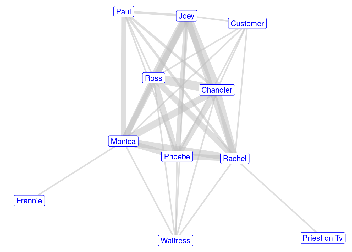
Figure 4.11: Visualization of the network of characters in Episode 1 of Friends, based on characters speaking in the same scene together
4.2.3 Approaches in Python
To repeat the work in the previous sections in Python, we will use the BeautifulSoup package to scrape our web script of the first episode of Friends.
import requests
from bs4 import BeautifulSoup

url = "https://fangj.github.io/friends/season/0101.html"
script = requests.get(url)

# parse the html of the page
friends_ep1 = BeautifulSoup(script.text, "html.parser")
The object friends_ep1 contains all the HTML code of the script webpage. Now we need to look for the string Scene: and replace it with the string <b>New Scene:</b>. It should be clear soon why we should put the replacement string in bold HTML tags.
originalString = "Scene:"
replaceString = "<b>New Scene:</b>"
friends_ep1_replace = BeautifulSoup(str(friends_ep1)\
.replace(originalString, replaceString))
Now we know from viewing the webpage or inspecting the HTML code that the characters’ names who are speaking in scenes will be inside bold or strong HTML tags. So, first let’s get everything that is in bold or strong tags in the document, and then let’s match for any alphabetic string (including spaces) prior to a colon using regular expression syntax. This should include the New Scene tags that we created in the last step.
# use re (regular expressions) package
import re

# find everything in bold tags with alpha preceding a colon
searchstring = re.compile("^[A-Za-z ]+(?=:)")
friends_ep1_bold = friends_ep1_replace.find_all(['b', 'strong'],
text = searchstring)

# extract the text and remove colons
friends_ep1_list = [friends_ep1_bold[i].text.replace(':', '')
for i in range(0, len(friends_ep1_bold) - 1)]

# check first few unique values returned
sorted(set(friends_ep1_list))[0:7]
## ['All', 'Chandler', 'Chandler ', 'Customer', 'Frannie', 'Joey', 'Monica']This looks promising; now we need to get rid of the ‘All’ entries and any entries containing ‘and’.
friends_ep1_list2=[entry.strip() for entry in friends_ep1_list
if "All" not in entry and " and " not in entry]

# check first few entries
sorted(set(friends_ep1_list2))[0:7]
## ['Chandler', 'Customer', 'Frannie', 'Joey', 'Monica', 'New Scene', 'Paul']Now we are ready to organize our characters by scene. First, we do a scene count, then we create a dataframe and obtain unique character lists by scene.
import pandas as pd

# number scene by counting previous "New Scene" entries and adding 1
scene_count = []

for i in range(0,len(friends_ep1_list2)):
  scene_count.append(friends_ep1_list2[0:i+1].count("New Scene"))

# create a pandas dataframe
df = {'scene': scene_count, 'character': friends_ep1_list2}
scenes_df = pd.DataFrame(df)

# remove New Scene rows
scenes_df = scenes_df[scenes_df.character != "New Scene"]

# get unique characters by scene
scenes = scenes_df.groupby('scene')['character'].unique()

# check
scenes.head()
## scene
## 1 [Monica, Joey, Chandler, Phoebe, Ross, Rachel,...
## 2 [Monica, Chandler, Ross, Rachel, Phoebe, Joey,...
## 3 [Phoebe]
## 4 [Ross, Joey, Chandler]
## 5 [Monica, Paul]
## Name: character, dtype: objectNow we need to create a function to find all unique pairs inside a scene character list. Here’s one way to do it:
import numpy as np

# define function
def unique_pairs(chars: object) -> pd.DataFrame:
  # start with uniques
  characters = np.unique(chars)
  # create from-to list dataframe
  char1 = []
  char2 = []
  df = pd.DataFrame({'char1': char1, 'char2': char2})
  # iterate over each entry to form pairs
  if len(characters) > 1:
    for i in range(0, len(characters) - 1):
      char1 = [characters[i]] * (len(characters) - i - 1)
      char2 = [characters[i] for i in range(i + 1, len(characters))]
      # append to dataframe
      df2 = pd.DataFrame({'char1': char1, 'char2': char2})
      df = df.append(df2, ignore_index = True)
  return df

# test on scene 11
unique_pairs(scenes[11])
## char1 char2
## 0 Chandler Joey
## 1 Chandler Monica
## 2 Chandler Paul
## 3 Chandler Rachel
## 4 Joey Monica
## 5 Joey Paul
## 6 Joey Rachel
## 7 Monica Paul
## 8 Monica Rachel
## 9 Paul RachelThis looks right. Now we need to apply this to every scene and gather the results into one DataFrame.
# start DataFrame
char1 = []
char2 = []

edgelist_df = pd.DataFrame({'char1': char1, 'char2': char2})

for scene in scenes:
  df = unique_pairs(scene)
  edgelist_df = edgelist_df.append(df, ignore_index = True)
Now we can order across the rows alphabetically and count the occurrences of each unique character pair to get our edge weights.
# sort each row alphabetically
edgelist_df = edgelist_df.sort_values(by = ['char1', 'char2'])

# count by unique pair
edgelist = edgelist_df.groupby(['char1', 'char2']).\
apply(len).to_frame("weight").reset_index()

# check
edgelist.head()
## char1 char2 weight
## 0 Chandler Customer 1
## 1 Chandler Joey 8
## 2 Chandler Monica 6
## 3 Chandler Paul 2
## 4 Chandler Phoebe 5This is what we need to create and visualize our graph of Episode 1 of Friends, which can be seen in Figure 4.12 with the edge thickness determined by edge weight.
import networkx as nx
from matplotlib import pyplot as plt

# create networkx object
friends_ep1_network = nx.from_pandas_edgelist(edgelist,
source = "char1", target = "char2", edge_attr=True)

# visualize with edge weight as edge width
np.random.seed(123)
weights = list(
  nx.get_edge_attributes(friends_ep1_network, 'weight').values()
)
nx.draw_networkx(
  friends_ep1_network, node_color = "lightblue", node_size = 60,
  edge_color = "grey", with_labels = True, width = np.array(weights)
)
plt.show()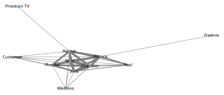
Figure 4.12: Graph of Friends character network from Episode 1 with edge width indicating the number of shared scenes
4.3 Learning exercises
4.3.1 Discussion questions
- What kinds of data sources are most likely to already exist in a graph-friendly form? Why?
- What are the two most important things to define when you intend to transform data into a graph-friendly structure?
- Imagine that you are working in a global law firm with a database that has three tables. One table lists employee location details including office and home address. A second table includes details on which clients each employee has been working for and what specialty areas they focus on with each client. A third table lists the education history of each employee including school and major/subject area. List out or sketch all the different ways you can think to turn this data into a graph.
- Pick one or two of your answers from Question 3 and write down two options for how to structure a graph for each of them. For one option, consider a graph where employees are the only vertices. Then consider a graph where there are at least two different entity types as vertices.
- Considering your answers to Question 4, how might your edges be defined in each of your options? Would the edges have any properties?
For the examples in Questions 6-10, discuss ways that information could be extracted, reshaped and loaded into a graph in order to serve a useful analytic purpose.
- Loyalty card data for a retail company showing detailed information on customer visits and purchases.
- Data from the calendars of a large number of company employees.
- Data from automatic number plate scanning from police cameras on major roads in a large city.
- Data on addresses of deliveries made by a courier company.
- Electronic files of legal contracts between different organizations to deliver specified services at specified prices.
4.3.2 Data exercises
Load the park_reviews data set from the onadata package or download it from the internet43. This data contains the reviews of a collection of Yelp users on dog parks in the Phoenix, Arizona area.
- Create an edgelist and vertex set that allows you to build a graph showing both the parks and the users as entity types. Include the
starsrating as an edge property and ensure that entity types are distinguishable in your data. - Use your edgelist and vertex set to create a graph object that has edge and vertex properties.
- Visualize your graph in a way that differentiates between users and parks. Use your visualization to point out users that have reviewed numerous dog parks.
- Generate a subgraph consisting only of edges where the
starsrating was 5. Repeat your visualization for this subgraph. Use it to identify a frequently 5-star rated park. Has any user reviewed more than one park as 5-star rated?
Go to the webpage containing the script for Season 1, Episode 2 of Friends at https://fangj.github.io/friends/season/0102.html.
- Repeat the steps in Section 4.2 to scrape this webpage to obtain a list of scenes and characters speaking in each scene. Watch out for any additional cleaning that might be necessary for this script compared to the Episode 1 script.
- Use the methods in Section 4.2, including the
unique_pairs()function, to create an edgelist for the character network for Episode 2 with the same edge weight based on the number of scenes in which the characters both spoke. - Create a graph for Episode 2 and visualize the graph.
- Combine the edgelist for both Episodes 1 and 2 by adding the weights for each character pair, and then create and visualize a new graph that combines both episodes.
- Extension: Try to wrap the previous methods in a function that creates an edgelist for any arbitrary Friends episode found at
https://fangj.github.io/friends/. Add more cleaning commands for unexpected formatting that you might see in different scripts. - Extension: Try to run your function on all Season 1 episodes of Friends and use the results to create and visualize a graph of the character network of the entire first season.
You can find and download the full version of the Chinook open-source SQLite database at https://www.sqlitetutorial.net/sqlite-sample-database/↩︎
The limited cleaning commands here work for this specific episode, but they would need to be expanded to be used on more episodes to take into account any unpredictable formatting in the scripts. The reality of most scraping exercises is that some code has to be written to deal with exceptions.↩︎