6 Vertex Importance and Centrality

Keith McNulty

It follows from much of the earlier work we have been doing in this book that the vertices of a graph can provide rich information about a network, its structure and its dynamics. In sociology and psychology contexts, this is particularly true, because more often than not vertices represent people. The fact that people play different roles and have different influences inside groups and communities has motivated centuries of sociological and psychological research, so it is unsurprising that the concept of vertex importance and influence is of great interest in the study of people or organizational networks.

But importance and influence are not precisely defined concepts, and to make them real within the context of graphs and networks we need to find some sort of mathematical definition for them. In many visual graph layouts, more important or influential vertices that have stronger roles in overall connectivity will usually be positioned toward the center of a group of other vertices⁵³. Intuitively therefore, we use the term ‘centrality’ to describe the importance or influence of a vertex in the connected structure of a graph.

In this chapter we will go through the most common types of centrality that can be measured for vertices in graphs, and discuss how they can be interpreted in the context of people or organizational networks. We will show how to calculate different types of centrality in R or Python and how to illustrate centrality in graph visualizations. We will then reprise our example of the French office building network from the previous chapter to illustrate the utility of centrality in network analysis.

In this chapter we will use the $G_{14}$ graph which we introduced in the previous chapter, which is an undirected and unweighted graph. Most centrality measures are valid and easily calculated for directed graphs, and will depend on defining the direction of the edges to consider. Figure 6.1 shows the $G_{14}$ graph with four vertices of interest colored differently from other vertices.

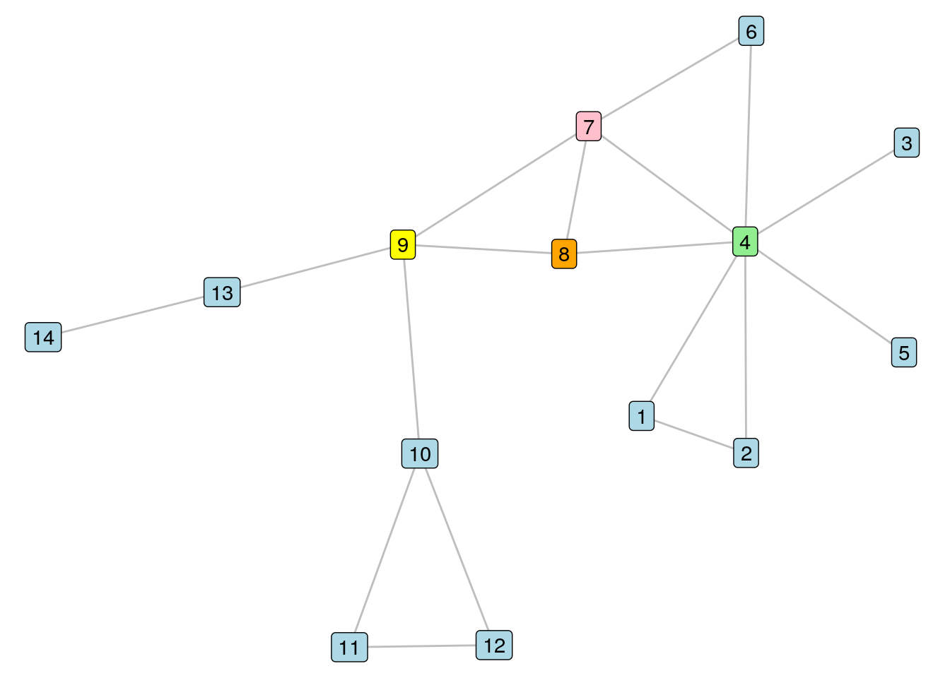
$The $G_{14}$ graph with four vertices of interest colored differently$

Figure 6.1: The $G_{14}$ graph with four vertices of interest colored differently

6.1 Vertex centrality measures in graphs

As we look at the $G_{14}$ graph in Figure 6.1, we see that the colored nodes seem to occupy prominent roles in the connective structure of the graph. If we removed Vertex 9, for example, we would split our graph into three disconnected components. Vertex 4 seems to be connected to a lot of immediate neighbors, and we would also split the graph if we removed it, leaving behind some isolates⁵⁴. Vertex 7 seems to occupy a stealthy position from which to efficiently reach other vertices, while Vertex 8 seems to sit in between those other three and probably can’t be ignored for that reason alone.

What if these vertices represented people in an organization? Would the departure of Vertex 4 mean that Vertices 1, 2, 3 and 5 lose their entire connection to the remainder of the organization? Would the departure of Vertex 9 split the organization in terms of the flow of work? If we wanted to distribute important information across the organization by means of these connections, which vertex would be a good place to start? By understanding centrality we can start to appreciate the possible impact of changes to the network, or identify important or influential actors in the network.

6.1.1 Degree centrality

The degree centrality or valence of a vertex $v$ is the number of edges connected to $v$. Alternatively stated, in an unweighted and undirected graph it is simply the number of neighbors of $v$ or the number of vertices of distance 1 from $v$. For example, the degree centrality of Vertex 8 in $G_{14}$ is 3, and for Vertex 4 it is 7. It should not be difficult to see that Vertex 4 has the highest degree centrality in $G_{14}$.

Degree centrality is a measure of immediate connection in a network. It could be interpreted as immediate reach in a social network. Its precise interpretation depends strongly on the nature of the connection. In a network of academic co-authoring, someone with high degree centrality has collaborated directly with a larger number of other academics. In our French office building network from Section 5.3, someone of high degree centrality is likely to be well-known socially to a greater number of colleagues.

Related to degree centrality is ego size. The $n$-th order ego network of a given vertex $v$ is a set including $v$ itself and all vertices of distance at most $n$ from $v$. The $n$-th order ego size is the number of vertices in the $n$-th order ego network. In $G_{14}$, Vertex 8 has a 1st order ego size of 4, a 2nd order ego size of 11, and a third order ego size of 14 (the entire graph). It easily follows that the 1st order ego size of a vertex is one greater than the degree centrality of the vertex.

6.1.2 Closeness centrality

The closeness centrality of a vertex $v$ in a connected graph is the inverse of the sum of the distances from $v$ to all other vertices. Let’s take a moment to understand this better by looking at an example. We will calculate the closeness centrality of Vertex 8 from $G_{14}$. Vertex 8 has the following distances to other vertices:

Distance 1 to vertices 4, 7 and 9
Distance 2 to vertices 1, 2, 3, 5, 6, 10 and 13
Distance 3 to vertices 11, 12 and 14

The sum of these distances is 26, and the inverse of 26 is 0.038. Inverting this distance means that lower total distances will generate higher closeness centrality. Therefore, the vertex with the highest closeness centrality will be the most efficient in reaching all the other vertices in the graph. While Vertex 8 has one of the highest closeness centralities in $G_{14}$, Vertex 7 has a slightly higher closeness centrality, because its additional direct edge to Vertex 6 gives it a slightly lower total distance of 25 to the other vertices, and therefore a slightly higher closeness centrality of 0.04.

Closeness centrality is a measure of how efficiently the entire graph can be traversed from a given vertex. This is particularly valuable in the study of information flow. In social networks, information shared by those with high closeness centrality will likely reach the entire network more efficiently. In our French office building network from Section 5.3, those with high closeness centrality may be better choices for efficiently spreading a message through social interactions or word-of-mouth.

6.1.3 Betweenness centrality

The betweenness centrality of a vertex $v$ is calculated by taking each pair of other vertices $x$ and $y$, calculating the number of shortest paths between $x$ and $y$ that go through $v$, dividing by the total number of shortest paths between $x$ and $y$, then summing over all such pairs of vertices in the graph. We can use the following process to manually calculate this for Vertex 8 in $G_{14}$:

If we look at all pairs of Vertices 9 through 14, we conclude that Vertex 8 is not on any shortest paths between these vertices (betweenness centrality: 0).
Similarly for Vertices 1 through 7 we conclude that Vertex 8 is not on any of these shortest paths either (betweenness centrality: 0).
Now we look at all paths between Vertex 7 and Vertices 9 through 14, and conclude that Vertex 8 is not on any shortest paths for these pairs because Vertices 7 and 9 are adjacent (betweenness centrality: 0).
Now we look at all paths between Vertex 6 and Vertices 9 through 14, and conclude that Vertex 8 is not on any of these shortest paths, because a shorter route is through Vertex 7 (betweenness centrality: 0).
Finally, we look at all pairs between Vertices 1 through 5 and Vertices 9 through 14, and conclude that for each of the 30 such pairs there are two shortest paths, one of which goes through Vertex 7 and the other through Vertex 8 (betweenness centrality: $0.5 \times 30 = 15$).
Summing over these, we conclude that the betweenness centrality of Vertex 8 in $G_{14}$ is 15.

Using similar logic, it is not too difficult to reason that Vertex 9 has the highest betweenness centrality in $G_{14}$. If we split the graph on either side of Vertex 9, we have betweenness centralities of zero in the sets of vertices on each side, but any path between vertices on either side of Vertex 9 must pass through Vertex 9. There are 46 such paths between Vertices 1 through 8 and Vertices 10 through 14, and so the total betweenness centrality of Vertex 9 is 46.

Betweenness centrality is a measure of how important a given vertex is in connecting other pairs of vertices in the graph. It makes intuitive sense that Vertex 9 should have the highest betweenness centrality because its removal would have the largest destructive effect on overall connectivity in $G_{14}$, splitting it into a disconnected graph with three connected components. In people networks, individuals with higher betweenness centrality can be regarded as playing important roles in ensuring overall connectivity of the network, and if they are removed from the network the risks of overall disconnection are higher. This has strong applications in studying the effects of departures from organizations.

Playing around: It’s worth thinking about some of the things we did in the previous chapter based on our new understanding of degree, closeness and betweenness centrality. For example, how do certain types of central vertices influence the overall ‘closeness’ of a network? What would happen to average distance or edge density if we remove certain central vertices? Try playing around with removing Vertices 4 (highest degree centrality), 7 (highest closeness centrality) and 9 (highest betweenness centrality) from $G_{14}$ and determining the impact of these removals on diameter, mean distance and density.

6.1.4 Eigenvector centrality

The Eigenvector centrality or relative centrality or prestige of a vertex is a measure of how connected the vertex is to other influential vertices. It is impossible to define this without a little linear algebra.

Recall from Section 2.1.4 that the adjacency matrix $A = (a_{ij})$ for an unweighted graph $G$ containing $p$ vertices is defined as $a_{ij} = 1$ if $i$ and $j$ are adjacent vertices in $G$ and 0 otherwise. A vector $x = (x_1, x_2, ...,x_p)$ and scalar value $\lambda$ are considered an eigenvector and eigenvalue of $A$ if they satisfy the equation

\[ Ax = \lambda{x} \] If we require that $x$ can only have positive entries, then a unique solution exists to this equation which has maximum eigenvalue $\lambda$. We take $x$ and $\lambda$ for this solution and define the eigenvector centrality for vertex $v$ as

\[ \frac{1}{\lambda}\sum_{w \in G}a_{vw}x_w \]

Because this is solving for a system of linear equations with coefficients that relate to the connectedness of neighboring vertices, its solution is a measure of the relative influence of a vertex as a function of the influences of the vertices it is connected to. Vertices can have high influence through being connected to a lot of other vertices with low influence, or through being connected to a small number of highly influential vertices. Vertex 10 in $G_{14}$ has an eigenvector centrality of 0.12, and Vertex 2 has an eigenvector centrality of 0.23. This makes sense because Vertex 2 is connected to Vertex 4, which we already know has the highest degree centrality in the network. Intuitively, it shouldn’t be too hard to appreciate that Vertex 4 has the highest eigenvector centrality in $G_{14}$.

In directed graphs, eigenvector centrality gives rise to interesting measures of different types of influence. For example, imagine a citation network where certain authors are regularly citing a lot of influential articles. These authors are known as hubs, and their outgoing eigenvector centrality will be high. Hub score is the outgoing eigenvector centrality of a vertex. Meanwhile, authors who have high incoming eigenvector centrality will be frequently referenced by hubs, and these authors are known as authorities. Authority score is the incoming eigenvector centrality of a vertex. These types of measures are becoming increasingly adopted in fields such as bibliometrics. Note that in undirected graphs the hub score, authority score and eigenvector centrality of vertices are identical.

Playing around: We have not looked at the impact of edge weights on centrality in this chapter. This is because it is unusual to consider edge weights in centrality measures. Nonetheless, most centrality measures do have approaches to consider edge weights, and this is a topic of ongoing research. Usually in these situations, edge weights are transformed to be cost functions—for example by inverting them—so that edges with higher weights are considered ‘preferable’ in graph traversal. To see what I mean, go back and have a look at the $G_{14W}$ weighted graph from the previous chapter. Pick pairs of vertices and see what the shortest path between them would be using the sum of weights of edges, and what it would be using the sum of the inverse weights of edges.

6.2 Calculating and illustrating vertex centrality

6.2.1 Calculating in R

Degree centrality can be calculated for a specific set of vertices using the degree() function in igraph. By default, the degree centrality will be calculated for all vertices. Let’s load up our $G_{14}$ graph to demonstrate as we did in the previous chapter.

library(igraph)
library(dplyr)

# get g14 edgelist and ignore weights
g14_edgelist <- read.csv("https://ona-book.org/data/g14_edgelist.csv")
g14_unweighted <- g14_edgelist |> 
  dplyr::select(-weight)

# create g14 graph
g14 <- igraph::graph_from_data_frame(g14_unweighted, directed = FALSE)

# calculate degree centrality for all vertices
igraph::degree(g14)

##  9 10 11 13  8  4  6  1 12 14  7  2  3  5 
##  4  3  2  2  3  7  2  2  2  1  4  2  1  1

We can see that Vertex 4 has a degree centrality of 7, which agrees with our earlier manual calculations. Ego networks and ego sizes can be determined using the ego() and ego_size() functions.

# 2nd order ego network of Vertex 4
igraph::ego(g14, order = 2, nodes = "4")

## [[1]]
## + 9/14 vertices, named, from 857f25b:
## [1] 4 8 6 1 7 2 3 5 9

# size of ego network
igraph::ego_size(g14, order = 2, nodes = "4")

## [1] 9

Closeness centrality is calculated using the closeness() function for all or a subset of vertices. Let’s verify that this function returns the same results for Vertices 7 and 8 that we manually calculated earlier.

igraph::closeness(g14, vids = c("7", "8"))

##          7          8 
## 0.04000000 0.03846154

Betweenness centrality is calculated using the betweenness() function in a similar way. Let’s verify our previous manual calculations for Vertices 8 and 9.

igraph::betweenness(g14, v = c("8", "9"))

##  8  9 
## 15 46

Finally, eigenvector centrality can be calculated using the eigen_centrality() function. Note that this returns a list including various details about the computation⁵⁵. To see the actual centralities, you should call the vector element of the output list. Note also that this function scales the values by default so that the maximum eigenvector centrality is 1. To avoid this, set scale = FALSE.

eigens <- igraph::eigen_centrality(g14, scale = FALSE)
eigens$vector

##          9         10         11         13          8          4          6          1         12         14 
## 0.30157876 0.11585270 0.04773223 0.09618665 0.37800315 0.55038069 0.29000589 0.22676118 0.04773223 0.02806617 
##          7          2          3          5 
## 0.44350955 0.22676118 0.16059484 0.16059484

We can see confirmation here that Vertex 4 has the highest eigenvector centrality.

Playing around: There are a few other centrality-like measures available in igraph which you could explore and try to understand. Examples include page_rank() for Google’s measure of importance of a webpage, and hub_score() and authority_score() for directed networks. Consider testing these out on some data sets, like the wikivote data set from the onadata package or downloaded from the internet⁵⁶.

6.2.2 Calculating in Python

Again, as in the work in the previous chapter, centrality functions in networkx are very similar to those in igraph. The degree() function calculates degree centrality for all vertices by default, or you can specify a list of vertices.

import networkx as nx
import pandas as pd

# download edgelist and remove weights
g14_edgelist = pd.read_csv(
  "https://ona-book.org/data/g14_edgelist.csv"
)
g14_undirected = g14_edgelist.drop('weight', axis = 1)

# create undirected g14 graph
g14 = nx.from_pandas_edgelist(g14_undirected, source = 'from', 
target = 'to')

# calculate degree centrality of Vertices 4 and 9
nx.degree(g14, [4, 9])

## DegreeView({4: 7, 9: 4})

There are also methods called degree() for a Graph() object as well as in_degree() and out_degree() for DiGraph() objects in networkx.

g14.degree(4)

## 7

The ego network of a vertex can be obtained using the ego_graph() function. To obtain the 2nd order ego network of Node 4:

ego_4_2 = nx.ego_graph(g14, n = 4, radius = 2)
ego_4_2.nodes

## NodeView((9, 8, 7, 4, 6, 1, 2, 3, 5))

Closeness centrality is calculated using the closeness_centrality() function. However, in networkx this is normalized by multiplying the result by $n - 1$ where $n$ is the number of vertices in the graph. To obtain non-normalized closeness centrality, it will be necessary to divide the output of this function by $n - 1$.⁵⁷

# get non-normalized closeness centrality for Vertex 7
norm_closeness = nx.closeness_centrality(g14, 7)
norm_closeness/(len(g14.nodes) - 1)

## 0.04

Betweenness centrality is calculated using the betweenness_centrality() function. Again this is normalized by default but this can be set to False in the arguments⁵⁸. This function calculates values for all nodes and returns them in a dict.

# get non-normalized betweenness centrality for Vertex 9
between = nx.betweenness_centrality(g14, normalized = False)
between.get(9)

## 46.0

Finally, eigenvector centrality is calculated using the eigenvector_centrality() function, with a dict returned similar to betweenness_centrality().

eigen = nx.eigenvector_centrality(g14)
eigen.get(4)

## 0.5503779695532801

Closeness, betweenness and eigenvector centrality are calculated using incoming edges in networkx digraphs. To calculate the outgoing equivalent, simply use the reverse() method on the digraph to make all outgoing edges incoming and vice versa.

Playing around: networkx has a very wide range of centrality measures available. Visit the Centrality section of its documentation⁵⁹ and have a look at the options. Many of these are very specific to graph use cases in different industries and disciplines, but see if you can understand them and even give them a try with a data set.

6.2.3 Illustrating centrality in graph visualizations

As we reviewed in Chapter 3, we will often make adjustments when visualizing graphs to illustrate certain aspects of the graph’s structure. For example, we highlight certain vertices with color or adjust the thickness of certain edges. When we want to visually illustrate the importance or influence of vertices in graphs, we will often do so using centrality measures. The two most common methods are to adjust vertex size according to centrality or to use a centrality-related color scale. We will illustrate a couple of examples using ggraph in R to show some of the options available.

For greatest efficiency, it’s always a good idea to add centralities as vertex properties in graphs. Let’s add a few of these now in our $G_{14}$ graph.

V(g14)$degree <- degree(g14)
V(g14)$betweenness <- betweenness(g14)
V(g14)$eigen <- eigen_centrality(g14)$vector

Now we can create a visualization where we map the size of vertices to the degree vertex property, as in Figure 6.2. Note the scale_size() function which is useful for setting a scale to suit your visualization.

set.seed(123)
ggraph(g14, layout = "lgl") +
  geom_edge_link(color = "grey", alpha = 0.7) +
  geom_node_point(aes(size = degree), color = "lightblue",
                  show.legend = FALSE) +
  scale_size(range = c(5,15)) +
  geom_node_text(aes(label = name)) +
  theme_void()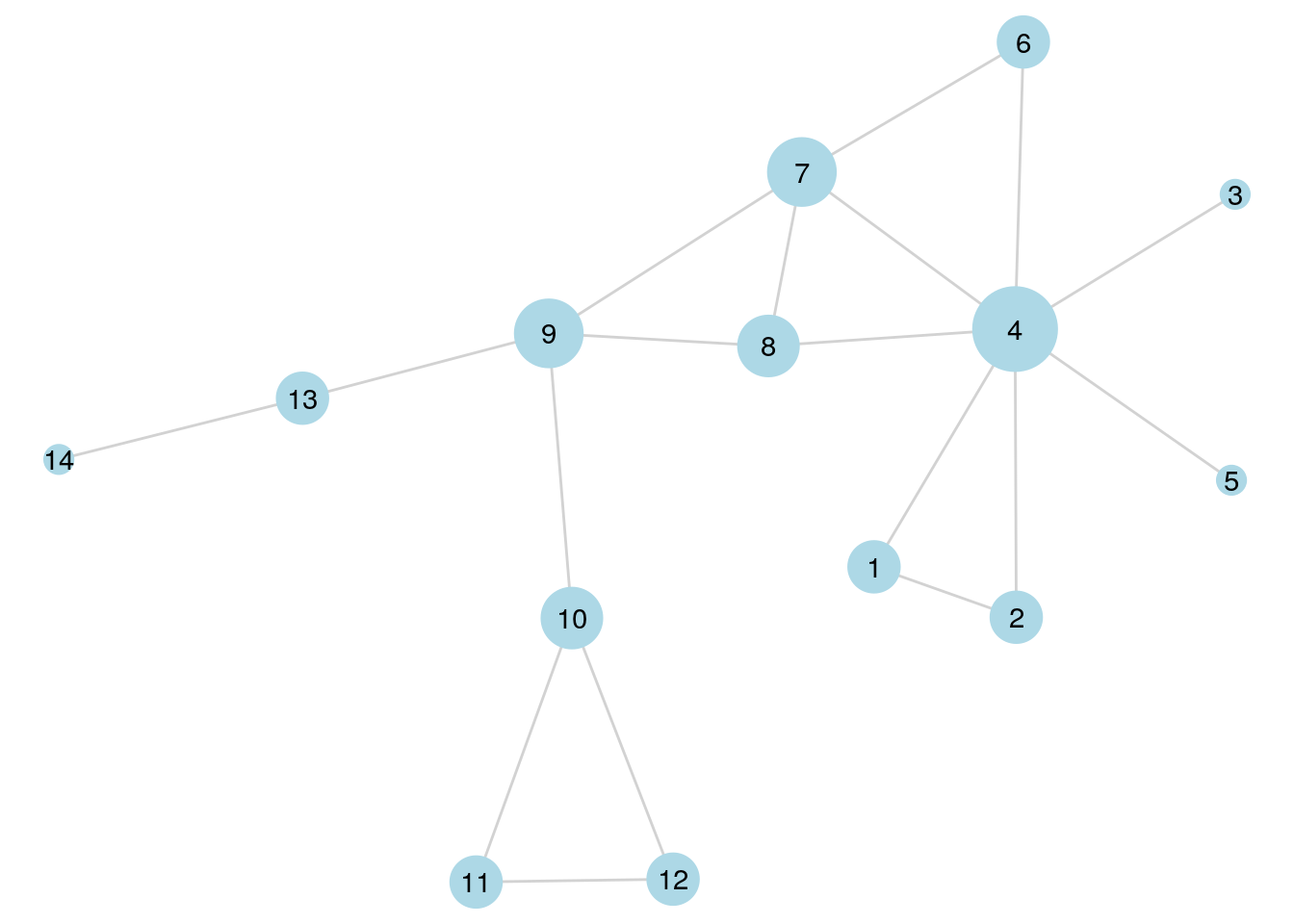

$$G_{14}$ with vertex size scaled according to degree centrality$

Figure 6.2: $G_{14}$ with vertex size scaled according to degree centrality

Alternatively, Figure 6.3 shows the same graph with the vertex colors scaled according to normalized eigenvector centrality. This helps us see that the vertices to the left of Vertex 9 in $G_{14}$ do not have particularly influential connections compared to those to the right.

set.seed(123)
ggraph(g14, layout = "lgl") +
  geom_edge_link(color = "grey", alpha = 0.7) +
  geom_node_point(size = 6, aes(color = eigen)) +
  scale_color_gradient(low = "lightblue", high = "red") +
  geom_node_text(aes(label = name)) +
  theme_void()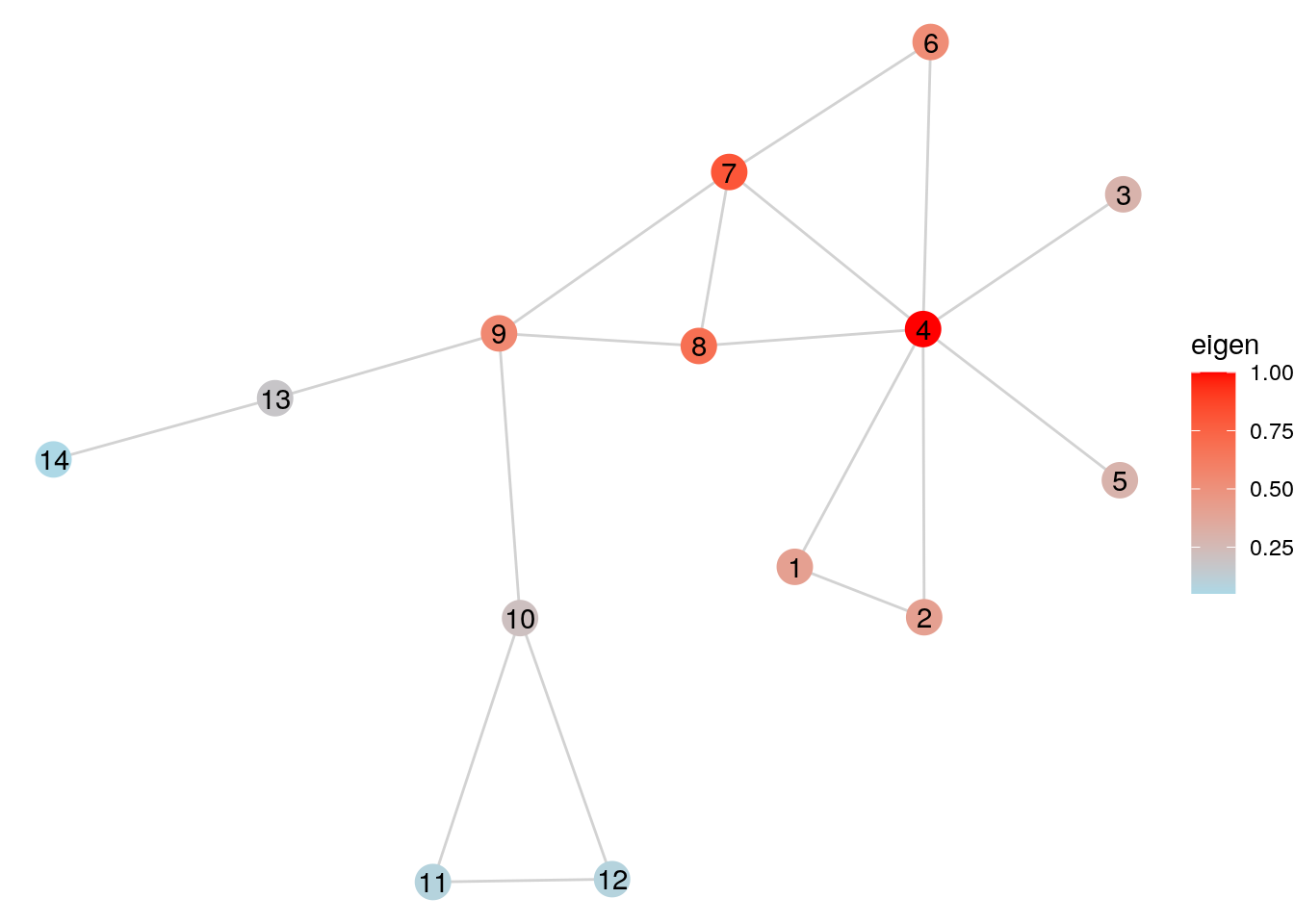

$$G_{14}$ with vertex size scaled according to normalized eigenvector centrality$

Figure 6.3: $G_{14}$ with vertex size scaled according to normalized eigenvector centrality

Playing around:. Play around with different ways of visualizing the centralities of vertices in $G_{14}$. Try using color, size or both. And also try the different types of centrality to see if the look of the graph changes substantially between them.

6.3 Examples of uses

In this section we will reprise the workfrance unweighted graph from the previous chapter and will use it to illustrate some common uses for centrality measures. First, we will look at how to find network-wide and department level ‘superconnectors’, then we will look at how to find potential socially influential actors in a network. Let’s load up the workfrance graph again.

set.seed(123)

# download workfrance data sets
workfrance_edges <- read.csv(
  "https://ona-book.org/data/workfrance_edgelist.csv"
)
workfrance_vertices <- read.csv(
  "https://ona-book.org/data/workfrance_vertices.csv"
)

# create graph
workfrance <- igraph::graph_from_data_frame(
    d = workfrance_edges,
    vertices = workfrance_vertices,
    directed = FALSE
)

6.3.1 Finding ‘superconnectors’

Individuals with high betweenness centrality in people networks could be regarded as ‘superconnectors’. Superconnectors can play very valuable roles in the social integration of new entrants to the network, and they can also present greater risk of connective disruption if they leave the network. Imagine a new hire is about to join the DMI department in our workfrance network. We want to assign two ‘buddies’ to this individual to help them socially integrate into the workplace more effectively. Given that it is important for the individual to assimilate into their own department and into the workplace as a whole, we want to select the best two current employees to assist with both goals. Let’s start with the DMI department first.

In order to study the DMI department as a self-contained network, we will create an induced subgraph which contains only those in that department and the connections between them, and visualize this network, labeling the employee IDs, as in Figure 6.4.

# create DMI subgraph
DMI_vertices <- V(workfrance)[V(workfrance)$dept == "DMI"]
DMI_graph <- igraph::induced.subgraph(workfrance, vids = DMI_vertices)

# visualize
set.seed(123)
ggraph(DMI_graph) +
  geom_edge_link(color = "grey", alpha = 0.7) +
  geom_node_point(color = "lightblue", size = 4) +
  geom_node_text(aes(label = name), size = 2) + 
  theme_void()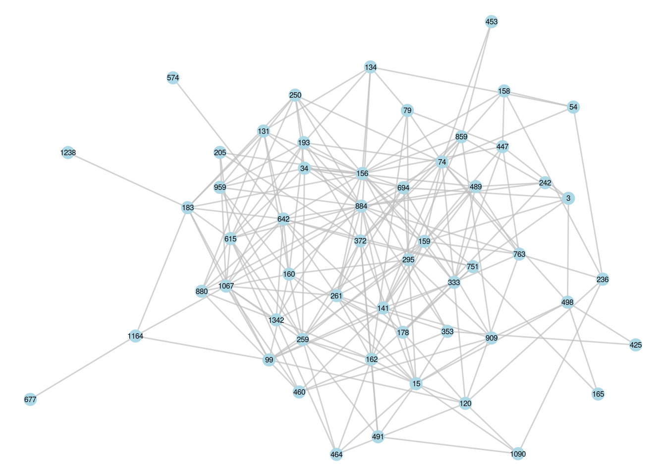

Figure 6.4: The induced subgraph of the DMI department in our French workplace

Now we are interested in those who have the strongest role in connecting others in this network. Let’s find the top three individuals in terms of betweenness centrality.

# get IDs of top 3 betweenness centralities
ranked_betweenness_DMI <- DMI_graph |> 
  betweenness() |> 
  sort(decreasing = TRUE) 

(top3_DMI <- names(ranked_betweenness_DMI[1:3]))

## [1] "156" "74"  "884"

These are the IDs of the top three superconnectors in the DMI department. Now we can visualize the graph again, but let’s adjust vertex size by betweenness and color the top 3 superconnectors, as in Figure 6.5.

# add betweenness vertex property
V(DMI_graph)$betweenness <- betweenness(DMI_graph)

# add top three superconnectors property
V(DMI_graph)$top3 <- ifelse(V(DMI_graph)$name %in% top3_DMI, 1, 0)

# visualize
set.seed(123)
ggraph(DMI_graph) +
  geom_edge_link(color = "grey", alpha = 0.7) +
  geom_node_point(aes(color = as.factor(top3), size = betweenness),
                  show.legend = FALSE) +
  scale_color_manual(values = c("lightblue", "pink")) +
  geom_node_text(aes(label = name), size = 2) + 
  theme_void()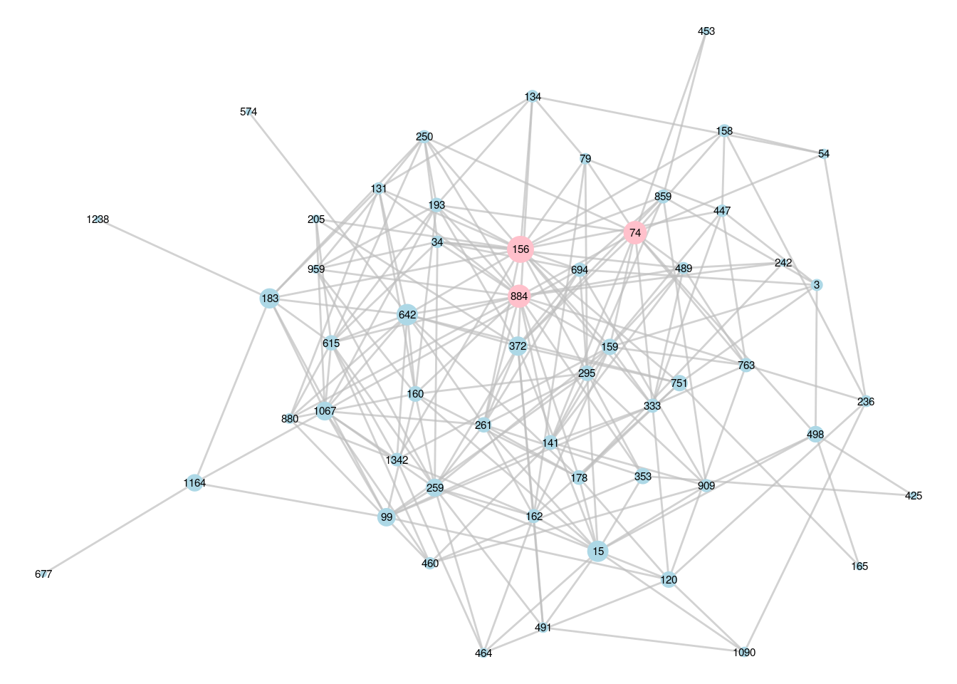

Figure 6.5: DMI subgraph with the top three superconnectors identified

In a similar way, we can find the superconnectors of the overall workfrance network.

# get IDs of top 3 betweenness centralities
ranked_betweenness_workfrance <- workfrance |> 
  betweenness() |> 
  sort(decreasing = TRUE) 

#get top 3
(top3_workfrance <- names(ranked_betweenness_workfrance[1:3]))

## [1] "603" "99"  "322"

In Figure 6.6, we create a graph of the workfrance network with vertex size scaled by betweenness centrality. We color by department so we can easily see which departments our superconnectors are in.

# add betweenness property
V(workfrance)$betweenness <- betweenness(workfrance)

# label only if a top 3 superconnector
V(workfrance)$btwn_label <- ifelse(
  V(workfrance)$name %in% top3_workfrance,
  V(workfrance)$name, 
  ""
)

# visualize
set.seed(123)
ggraph(workfrance) +
  geom_edge_link(color = "grey", alpha = 0.7) +
  geom_node_point(aes(color = dept, size = betweenness),
                  show.legend = FALSE) +
  geom_node_text(aes(label = btwn_label), size = 4) + 
  theme_void()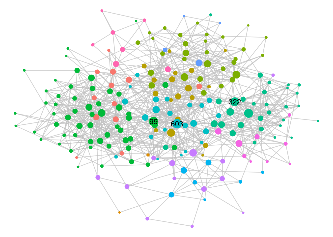

Figure 6.6: French workplace graph with the top 3 superconnectors identified

We can see upon examination that our top 3 organization-wide superconnectors are all in different departments. Putting all this together, it would seem that a good choice of buddies for the new hire would be employee 156 for departmental integration and employee 603 for office-wide integration, although any combination of the six individuals identified through this analysis would probably be decent choices.

6.3.2 Identifying influential employees

Influential actors in a network can be very useful to identify. In organizational contexts, working with more influential employees can make a difference to how certain initiatives or changes can be perceived by other employees. Influential employees can also be useful in efficiently tapping into prevalent opinions across the entire employee population. Imagine that we want to identify individuals from across the organization to participate in important workshops to problem solve some critical operational initiatives. These initiatives will affect employees at both an overall and a department level; therefore, it would be ideal to have individuals who are influential within each department as well as across the entire organization.

Again, let’s look at a single department—the DMI department—as an example. Because we are interested in overall influence, this could mean we are equally interested in employees with a lot of connections or employees who are ‘stealthily’ influential in being connected to a smaller number of other highly connected employees. The best measure for this is eigenvector centrality.

First we identify the top three most influential individuals in the DMI department as measured by eigenvector centrality by working on the DMI subgraph.

# working with lists so use purrr package
library(purrr)

# get IDs of top 3 eigen centrality
ranked_eigen_DMI <- DMI_graph |> 
  eigen_centrality() |> 
  pluck("vector") |> 
  sort(decreasing = TRUE)

#get top 3
(top3_DMI_eigen <- names(ranked_eigen_DMI[1:3]))

## [1] "884" "156" "642"

We see two employee IDs that are in common with our top 3 superconnectors. We can also identify the top 3 most influential individuals across the workfrance graph according to their eigenvector centrality.

# get IDs of top 3 eigen centrality
ranked_eigen_workfrance <- workfrance |> 
  eigen_centrality() |> 
  pluck("vector") |> 
  sort(decreasing = TRUE)

#get top 3
(top3_workfrance_eigen <- names(ranked_eigen_workfrance[1:3]))

## [1] "603" "649" "147"

We see one individual in common with our top 3 superconnectors. Let’s visualize this network so we can identify the department mix of our top 3 most influential individuals, as in Figure 6.7.

# add betweenness property
V(workfrance)$eigen <- eigen_centrality(workfrance)$vector

# label only if a top3 superconnector
V(workfrance)$eigen_label <- ifelse(
  V(workfrance)$name %in% top3_workfrance_eigen,
  V(workfrance)$name, ""
)

# visualize
ggraph(workfrance) +
  geom_edge_link(color = "grey", alpha = 0.7) +
  geom_node_point(aes(color = dept, size = eigen),
                  show.legend = FALSE) +
  geom_node_text(aes(label = eigen_label), size = 4) + 
  theme_void()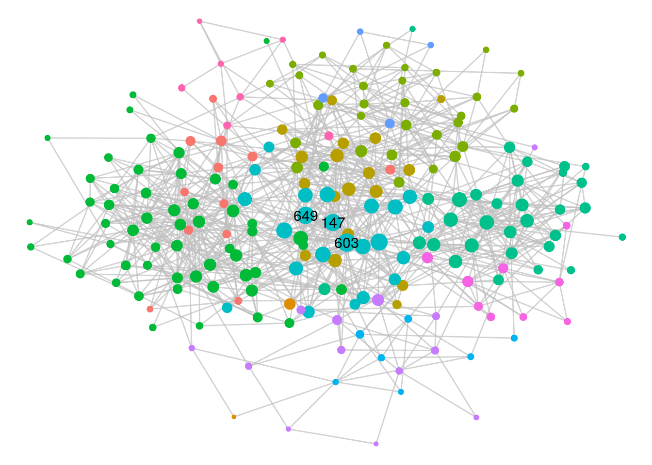

Figure 6.7: French workplace graph with the top 3 most influential vertices identified

This time we see that our three most influential individuals are all in the same department, suggesting that this department may be a strategically important one to involve in any planned change initiatives.

6.4 Learning exercises

6.4.1 Discussion questions

Describe the general concept of vertex centrality in networks and why it is important.
Define the degree centrality of a vertex $v$ in an undirected graph $G$ in at least two different ways. How would you interpret the degree centrality of $v$ in an organizational network? Manually calculate the degree centrality of Vertices 9, 10 and 11 in $G_{14}$.
Draw the 2nd order ego network of Vertex 8 in $G_{14}$. What is the 2nd order ego size of Vertex 8?
Define closeness centrality and describe how it can be interpreted. Manually calculate the closeness centrality of Vertex 10 in $G_{14}$ (feel free to express your answer as a fraction).
Define betweenness centrality and describe how it can be interpreted. Manually calculate the betweenness centrality of Vertex 4 in $G_{14}$.
Describe how you would interpret the eigenvector centrality of a vertex in an undirected graph $G$.
For each of the four main centrality measures—degree, closeness, betweenness and eigenvector—write down some potential benefits from knowing which individuals rank highest in a people network.
When visualizing graphs, name some ways to illustrate vertex centrality.
Why might some centrality functions in R or Python not actually output the raw centrality measure? Give an example of this. Do you think it matters? What would you do to correct it if you need to?
Describe some additional considerations in the calculation of vertex centrality in the case of directed graphs and in the case of weighted graphs.

6.4.2 Data exercises

Use an appropriate function to calculate the degree centrality of Vertices 9, 10 and 11 in $G_{14}$ and verify that the output matches your manual calculations from the earlier questions.
Create and visualize the 2nd order ego network of Vertex 8 in $G_{14}$.
Use an appropriate function to calculate the closeness centrality of Vertex 10 in $G_{14}$ and verify that it agrees with your manual calculation from the earlier questions.
Use an appropriate function to calculate the betweenness centrality of Vertex 4 in $G_{14}$ and verify that it agrees with your manual calculation from the earlier questions.
Find the mean eigenvector centrality of all vertices in $G_{14}$. Do this twice, raw and normalized.
Visualize $G_{14}$ with the size of the vertices scaled to their eigenvector centrality and the color scaled to their closeness centrality.

For questions 6 to 10, create an undirected graph from the Facebook friendships in the schoolfriends_edgelist and schoolfriends_vertices data sets in the onadata package or downloaded from the internet⁶⁰. Recall from the exercises in Chapter 3 that this data contains information on friendships between students in a French high school. Make sure not to include the reported friendships in this graph. There are a lot of isolates in this graph because it only represents ‘known’ Facebook friendships, and you should remove isolates before proceeding⁶¹.

Identify the top 3 individuals with the most Facebook connections.
Determine 1st order and 2nd order ego sizes of the individual with the most Facebook connections. What proportion of the total connected population is included in these ego networks?
Plot the distribution of the degree centrality of all vertices using a histogram or density plot.
Identify which individuals have the maximum closeness centrality, betweenness centrality and eigenvector centrality in the graph. Visualize the network color coded by class and identify where these individuals are. What do you notice?
If you were the principal of this high school and were deciding class placements for next year, how might this information be useful to you?

Extension: For these questions, create a directed graph from the reported friendships in the same data set, and remove the isolates as before.

Identify the individuals with the maximum in-degree centrality and the maximum out-degree centrality in this network. How would you describe these two individuals in the friendship dynamics of the high school? Do you see anything in common with the Facebook friendships?
Calculate the hub scores and authority scores of the vertices. How would you interpret these?
Determine the 1st order ego network of the individual with the highest authority score. Visualize this as a directed network with vertices color coded by class. Do the same for the individual with the highest hub score. Can you use these visualizations to describe why these individuals have high authority/hub scores?

If you want to see an earlier example of this, take a look at Figure 3.8 for Zachary’s Karate Club network and note the positions of the influential actors, Mr Hi and John A.↩︎
Recall that isolates are vertices that are not connected to any other vertices.↩︎
For example, if you are curious to know the eigenvalue, you can look at the value element of the list↩︎
https://ona-book.org/data/wikivote.csv ↩︎
You may wonder why $n - 1$? This is simply the total number of other vertices that we are calculating the paths to. Strangely, there is no option to non-normalize in the arguments of this function as of recent versions of networkx. In any case, for the purposes of comparing vertices, it doesn’t matter a great deal whether you normalize or not.↩︎
The normalization here divides the result by the number of vertex pairs in a graph with $n-1$ vertices, which is $(n - 1)(n - 2)$ for directed graphs and $\frac{(n - 1)(n - 2)}{2}$ for undirected graphs.↩︎
https://networkx.org ↩︎
https://ona-book.org/data/schoolfriends_edgelist.csv and https://ona-book.org/data/schoolfriends_vertices.csv ↩︎
One easy way to identify isolates in a graph object G in R is to identify them using isolates <- which(degree(G) == 0), and then remove them using G_new <- remove.vertices(G, isolates).↩︎