8 Assortativity and Similarity
In this chapter we will round off our study of important graph concepts and metrics by looking at two new concepts which a people network analyst will often have good reason to study. The first concept is assortativity, and this is described as the tendency of vertices to connect or ‘attach’ to vertices with similar properties in a graph. This is effectively a measure of homophily in a network. Highly assortative networks are more robust to destructive events like the loss of vertices, but because of their concentration they can be inefficient in terms of information flow, and in organizational settings they can be problematic for diverse interaction and experience.
The second concept we will look at is vertex and graph similarity. In certain networks where information on vertex properties is not available, it may make sense to infer that two vertices are similar in some way if their immediate networks are very similar. The concept of similarity can be also extended to entire graphs. In the simplest case, we may be looking at the same set of vertices but using different definitions of connection, and we want a measure of whether those different definitions produce substantially the same network or an entirely different network. As organizations start to mine many different forms of data to define connection (email, calendar, timesheet, document collaboration to name a few), it is becoming more and more important to understand the similarities or differences between the networks generated by these data sources.
8.1 Assortativity in networks
We have already seen in previous chapters that it is natural to want to study the extent to which vertices with similar ground truth properties are more densely connected in a graph. In Chapter 7, we looked at how politicians representing the same political parties connect to each other over Twitter, or how schoolchildren in the same class connect over Facebook. In the exercises at the end of that chapter, we looked at how researcher communities form over email either within or between ground truth research departments.
The assortativity coefficient of a graph is a measure of the extent to which vertices with the same properties connect to each other. It is a relatively recently defined metric and is defined slightly differently according to whether the property of interest is categorical (e.g., department or political party) or numeric (e.g., degree centrality). See Newman (2002) for a full description and mathematical definition.
The assortativity coefficient of a graph ranges between \(-1\) and \(1\), just like a correlation coefficient. Assortativity coefficients close to \(1\) indicate that there is very high likelihood of two vertices with the same property being connected. This is called an assortative network. Assortativity coefficients close to \(-1\) indicate that there is very low likelihood of two vertices with the same property being connected. This is called a disassortative network. Networks with assortativity coefficients close to zero are neither assortative nor disassortative and are usually described as having neutral assortativity.
8.1.1 Categorical or nominal assortativity
Let’s look at categorical assortativity first by bringing back two examples from the previous chapter. First, we look at our Facebook schoolfriends network and calculate the assortativity by class. In R, we can use the assortativity_nominal() function to calculate categorical assortativity (see the end of this chapter for Python implementations). Note that these functions expect a numeric vector to indicate the category membership.
library(igraph)

# get data
schoolfriends_edgelist <- read.csv(
  "https://ona-book.org/data/schoolfriends_edgelist.csv"
)
schoolfriends_vertices <- read.csv(
  "https://ona-book.org/data/schoolfriends_vertices.csv"
)

# create undirected Facebook friendships graph
schoolfriends_fb <- igraph::graph_from_data_frame(
  d = schoolfriends_edgelist |>
    dplyr::filter(type == "facebook"),
  vertices = schoolfriends_vertices,
  directed = FALSE
)

# calculate assortativity by class for Facebook friendships
igraph::assortativity_nominal(
  schoolfriends_fb,
  as.integer(as.factor(V(schoolfriends_fb)$class))
)
## [1] 0.3833667This suggests moderate assortativity, or moderate likelihood that students in the same class will be Facebook friends. Now let’s compare to ‘real’ reported friendships.
# create directed graph of reported friendships
schoolfriends_rp <- igraph::graph_from_data_frame(
  d = schoolfriends_edgelist |>
    dplyr::filter(type == "reported"),
  vertices = schoolfriends_vertices
)

# calculate assortativity by class for reported friendships
igraph::assortativity_nominal(
  schoolfriends_rp,
  as.integer(as.factor(V(schoolfriends_fb)$class))
)
## [1] 0.7188919We see substantially higher assortativity by class for reported friendships, indicating that being in the same class is more strongly associated with developing a reported school friendship.
Playing around: You may remember the concept of modularity which we introduced in Chapter 7. For categorical vertex properties, modularity and assortativity effectively measure similar concepts. Calculate the modularity for the Facebook schoolfriends by class and compare it to the assortativity. Also, play around with some prior data sets and calculate the assortativity of some of the communities we detected in Chapter 7. Recall also our example from Chapter 5 where we divided up the workfrance population to have tables with a good mix of different departments. If you completed that exercise, you may be interested to compare the assortativity of that population by department versus by table to get a measure of how successful you were at creating diverse tables.
8.1.2 Degree assortativity
The most common form of numerical assortativity is degree assortativity. A high degree assortativity is a measure of preferential attachment in organizations, where highly connected vertices are connected with each other and a large number of vertices with low degree make up the remainder of the network.
Again, let’s use our schoolfriends networks as an example to calculate degree assortativity in R.
# degree assortativity of Facebook friendships (undirected)
igraph::assortativity_degree(schoolfriends_fb)
## [1] 0.02462444# degree assortativity of reported friendships (directed)
igraph::assortativity_degree(schoolfriends_rp)## [1] 0.3098123We see that real-life friendships are moderately assortative in this data, whereas Facebook friendships are approximately neutral. This indicates that more popular students have a stronger tendency in real-life to be friends with other popular students.
Although it is a relatively recent concept, assortativity is a useful measure in understanding people or organizational networks. Highly assortative networks demonstrate resilience in that knowledge, community and other social capital are concentrated in a strong core, and disruptions such as departures of actors from those networks are less likely to affect the network as a whole. However, such networks also demonstrate characteristics which are counterproductive to diversity and inclusion and can represent challenging environments for new entrants to adjust to.
It has been thought that social networks are unlike most other real life networks in that they are degree assortative. However, recent research has begun to question this. Although it does seem to be the case that social networks are more assortative than non-social networks, research on various data sets where the connection between individuals is direct (rather than inferred from joint membership of a group) suggests that social networks are likely neutrally assortative (Fisher et al. (2017)). This is a research topic of great interest currently in social network analysis.
8.2 Vertex similarity
Often we are not lucky enough to have really rich ground truth information on the vertices in a network. This is particularly the case if we need to analyze people networks under anonymization constraints. Nevertheless, as we have seen with examples in previous chapters like the workfrance graph and the ontariopol graph, computational methods allow us to infer conclusions about vertices and groups of vertices that can often be good estimates of the ground truth properties of those vertices. In some networks, we can conclude that vertices are similar in some way if they share very similar immediate connections. For example, in our workfrance graph, if two vertices have first degree networks that overlap to a large degree, it would not be unreasonable to infer a likelihood that those two vertices are from the same department.
The vertex similarity coefficient of a pair of vertices is a measure of how similar are the immediate networks of those two vertices. Imagine we have two vertices \(v_1\) and \(v_2\) in an unweighted graph \(G\). There are three common ways to calculate the vertex similarity of \(v_1\) and \(v_2\), as follows:
- The Jaccard similarity coefficient is the number of vertices who are neighbors of both \(v_1\) and \(v_2\) divided by the number of vertices who are neighbors of at least one of \(v_1\) and \(v_2\).
- The dice similarity coefficient is twice the number of vertices who are neighbors of both \(v_1\) and \(v_2\) divided by the sum of the degree centralities of \(v_1\) and \(v_2\). Thus, common neighbors are double counted in this method.
- The inverse log-weighted similarity coefficient is the sum of the inverse logs of the degrees of the common neighbors of \(v_1\) and \(v_2\). This definition asserts that common neighbors that have high degree in the network are ‘less valuable’ in detecting similarity because there is a higher likelihood that they would be a common neighbor simply by chance.
To illustrate these three types of vertex similarity coefficients and show how they are calculated in R, let’s bring back our \(G_{14}\) unweighted graph from Chapters 5 and 6, and visualize it again in Figure 8.1.
library(igraph)
library(ggraph)
library(dplyr)

# download edgelist and create unweighted graph
g14_edgelist <- read.csv("https://ona-book.org/data/g14_edgelist.csv")
g14 <- igraph::graph_from_data_frame(d = g14_edgelist |>
                                       dplyr::select(from, to),
                                     directed = FALSE)

# visualize
set.seed(123)
(g14viz <- ggraph(g14, layout = "lgl") +
    geom_edge_link(color = "grey") +
    geom_node_label(aes(label = name), fill = "lightblue") +
    theme_void())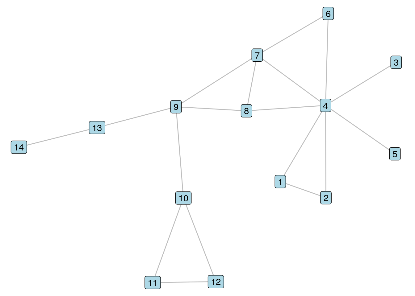
Figure 8.1: It’s our old friend \(G_{14}\) again
Let’s look at Vertices 7 and 8 in \(G_{14}\). To calculate the Jaccard similarity coefficient, we note that Vertices 4 and 9 are the two common neighbors of these vertices, and that Vertices 4, 6, 7, 8 and 9 are all neighbors of at least one of Vertices 7 and 8. Therefore, we should see a Jaccard similarity coefficient of 0.4. We use the similarity() function in igraph whose default is to calculate Jaccard similarity.
##      [,1] [,2]
## [1,]  1.0  0.4
## [2,]  0.4  1.0
We see in the off-diagonal components of this matrix confirmation of a Jaccard similarity coefficient of 0.4.
To calculate the dice similarity coefficient, we note that the sum of the degrees of Vertices 7 and 8 is 7; therefore, the dice similarity should equal \(\frac{4}{7}\) or 0.571.
##           [,1]      [,2]
## [1,] 1.0000000 0.5714286
## [2,] 0.5714286 1.0000000
Finally, to calculate the inverse log weighted similarity coefficient, we sum the inverse of the logs of the degrees of the common neighbors of Vertices 4 and 8, which is \(\frac{1}{\ln{7}} + \frac{1}{\ln{4}}\), which calculates to 1.235.
The output of this similarity() function variant returns the similarity of the selected vertices with all vertices in the network—try it if you like. In order to extract the specific similarity for Vertices 7 and 8, we should ensure to label the rows and columns of the matrix by vertex name before extracting a specific value from it.
# get invlogweighted similarity
invsim <- igraph::similarity(g14, method = "invlogweighted")

# rows and cols should be labelled by vertex name before extracting
colnames(invsim) <- V(g14)$name
rownames(invsim) <- V(g14)$name

# extract value for vertices 7 and 8
invsim["7", "8"]
## [1] 1.235246Playing around: Go back to some of our prior examples from Chapter 7 where we detected communities of more densely connected vertices in graphs like schoolfriends and ontariopol. Play around with calculating the similarity between pairs of vertices inside communities versus between communities and think about whether the results make sense.
8.3 Graph similarity
The general question of whether two graphs which contain vertices representing different entities still exhibit similar internal patterns and structures is of great interest in computer science and image recognition. The graph isomorphism problem, for example, is a computational problem concerned with finding a function that exactly maps the vertices of one graph onto other74.
In organizational network analysis we are usually more concerned with comparing graphs where the vertices represent the same entities (usually people), and where the vertex set is identical but where the edge set may be different. An example of this is our schoolfriends data set from earlier in this chapter, where the vertices are the same set of high school students, but where the edge sets are different according to whether the friendships are Facebook friendships or reported friendships. In this situation, we can use a common set similarity metric from set theory to determine how similar our graphs are.
Let \(G_1 = (V, E_1)\) and \(G_2 = (V, E_2)\) be two graphs with the same vertex set. The Jaccard similarity of \(G_1\) and \(G_2\) is the number of edges in both \(E_1\) and \(E_2\) divided by the number of edges in at least one of \(E_1\) and \(E_2\).
Note that a Jaccard similarity of 1 means that both graphs have identical edge sets and so are identical in structure, and a similarity of 0 means that both graphs have no edges in common. Let’s try this on our schoolfriends graphs. To do a fair comparison, we will redefine our Facebook schoolfriends graph to be a directed graph where edges always go in both directions.
# create directed version of Facebook graph
schoolfriends_fb_dir <- igraph::as.directed(schoolfriends_fb)
We can create a handy function to calculate the Jaccard similarity of the edge sets of two graphs. Note that the igraph package has special operators %s% for the intersection of two graphs (that is, all vertices and edges that both graphs have in common), and %u% for the union of two graphs (that is, all unique vertices and edges in both graphs combined).
# function for jaccard similarity of edge sets
jaccard_edgeset_similarity <- function(G1, G2) {
  inter <- length(E(G1 %s% G2))
  un <- length(E(G1 %u% G2))

  if (un == 0) {
    0
  } else {
    inter/un
  }
}


# test
jaccard_edgeset_similarity(schoolfriends_fb_dir, schoolfriends_rp)
## [1] 0.09727385We see that there is only about 10% similarity between the Facebook friendships and the ‘real’ reported friendships.
8.4 Calculating assortativity and similarity in Python
To demonstrate assortativity functions, we load up the schoolfriends data sets.
import networkx as nx
import pandas as pd

# load data
# get data
schoolfriends_edgelist = pd.read_csv(
  "https://ona-book.org/data/schoolfriends_edgelist.csv"
)
schoolfriends_vertices = pd.read_csv(
  "https://ona-book.org/data/schoolfriends_vertices.csv"
)

# create undirected facebook graph
schoolfriends_fb = nx.from_pandas_edgelist(
  df = schoolfriends_edgelist[
    schoolfriends_edgelist.type == 'facebook'
  ],
  source = "from",
  target = "to"
)

# create directed reported graph
schoolfriends_rp = nx.from_pandas_edgelist(
  df = schoolfriends_edgelist[
    schoolfriends_edgelist.type == 'reported'
  ],
  source = "from",
  target = "to",
  create_using=nx.DiGraph()
)

# add class vertex attribute to both graphs
class_attr = dict(zip(schoolfriends_vertices['id'],
schoolfriends_vertices['class']))
nx.set_node_attributes(schoolfriends_fb, name = "class",
values = class_attr)
nx.set_node_attributes(schoolfriends_rp, name = "class",
values = class_attr)
The following functions can be used to calculate categorical assortativity and degree assortativity, respectively.
## 0.3833666875368265## 0.7188918572576618## 0.024624435635859483## 0.30981226480406543To calculate Jaccard similarity between two vertices, we can use the jaccard_coefficient() function in networkx. In this example, we calculate the Jaccard coefficients for two pairs of vertices in schoolfriends_fb.
jaccards = nx.jaccard_coefficient(G = schoolfriends_fb,
ebunch = [(883, 132), (63, 991)])
sorted(jaccards)
## [(63, 991, 0.15384615384615385), (883, 132, 0.30612244897959184)]Dice similarity and inverse log weighted similarity coefficients can be calculated by creating functions.
# function for dice similarity
def dice_coefficient(G, ebunch = None):
      def dicesim(u, v):
        total_degree = nx.degree(G, u) + nx.degree(G, v)
        if total_degree == 0:
            return 0
        return 2*len(list(nx.common_neighbors(G, u, v))) / total_degree

      if ebunch is None:
        ebunch = nx.non_edges(G)
      return ((u, v, dicesim(u, v)) for u, v in ebunch)


# test
dice = dice_coefficient(G = schoolfriends_fb,
ebunch = [(883, 132), (63, 991)])
sorted(dice)
## [(63, 991, 0.26666666666666666), (883, 132, 0.46875)]import math
# function for inverse log weighted similarity
def invlogweight_coefficient(G, ebunch = None):
def invlogwsim(u, v):
logw = [1/math.log(nx.degree(G, w))
for w in nx.common_neighbors(G, u, v)]
if logw == 0:
return 0
return sum(i for i in logw)
if ebunch is None:
ebunch = nx.non_edges(G)
return ((u, v, invlogwsim(u, v)) for u, v in ebunch)
# test
invlogw = invlogweight_coefficient(G = schoolfriends_fb,
ebunch = [(883, 132), (63, 991)])
sorted(invlogw)## [(63, 991, 0.5728002621049868), (883, 132, 4.566433503199232)]Finally, to calculate Jaccard similarity of two edge sets, a simple function can be written:
# create function for Jaccard edge set similarity
def jaccard_edgeset_similarity(G1, G2):
  setG1 = set(G1.edges)
  intersection = len(setG1.intersection(G2.edges))
  union = len(setG1.union(G2.edges))

  if union == 0:
    return 0
  return intersection/union

# recreate schoolfriends_fb as directed graph to compare
schoolfriends_fb_dir = schoolfriends_fb.to_directed()

# test
jaccard_edgeset_similarity(schoolfriends_fb_dir, schoolfriends_rp)
## 0.097273853779429998.5 Learning exercises
8.5.1 Discussion questions
- Describe the meaning of the term ‘assortativity’ for vertices in a graph.
- Describe the meaning of degree assortativity and discuss how it relates to the concept of preferential attachment.
- Describe why assortativity and modularity are similar concepts in graph theory.
- Describe the concept of vertex similarity and define two measures of vertex similarity.
- Describe a method to compare the similarity of two graphs with the same vertex sets.
8.5.2 Data exercises
- Calculate the gender assortativity coefficient in the two
schoolfriendsgraphs. What would you conclude from this? - Calculate the department assortativity coefficient in the
workfrancegraph from earlier chapters. - Calculate the degree assortativity coefficient of the
workfranceand theontariopolgraphs from previous chapters. How would you describe the meaning of the difference between the two? - Choose pairs of vertices from the same department in the
workfrancegraph and calculate their Jaccard similarity coefficients. Then choose pairs from different departments and do the same. Do the results make sense? Why? - Find the three vertices with highest degree centrality in the
workfrancegraph, and calculate some pairwise similarity coefficients for them. Now do the same with three vertices with relatively low degree centrality. Do the results make sense? Why?
References
The question of whether the graph isomorphism problem can be solved in polynomial time is one of a number of high-profile open graph problems currently.↩︎