10 Bonus Chapter: Using Twitter for Network Analysis
Social media engines are by their very nature rich sources of data for modeling networks of friends, colleagues and other relationships. In Chapter 7 for example, we used data extracted from Twitter to study a network of Canadian politicians. Such data is not always easy to extract, as different social media companies have different philosophies about data access, and some make it very difficult for user data to be extracted.
However, Twitter is one of the more open platforms, and anyone who wants to can extract a certain amount of data from Twitter provided the user accounts they are interested in are public accounts. In this chapter we will go through how to extract data from Twitter and how to turn that data into a graph object for further study. As an example, we will extract data on the recent tweets of British politicians sitting in the House of Commons as at mid-2022 and we will use it to detect influential politicians, political party groupings and factions.
10.1 Accessing the Twitter API
The Twitter Application Programming Interface (API) allows an individual to access the database underlying Twitter and extract certain data from it. As of the time of writing, there are two versions of the API in operation - version 1.1 and the newer version 2. Here we will use version 1.1 of the API, as this is more established and will allow us to use helpful packages which have been written to make access easier.
In order to access the Twitter API, you need to have your own Twitter account and you need to use this account to sign up for a Twitter developer account at the Twitter Developer Platform. When you sign up for a developer account, you can set up a project and an application. Once you have done this, you can generate a series of access codes. For v1.1 of the API, you will need the API Key and Secret and the Access Token and Secret. Note that you will only be able to see and copy these once, so make sure you do so after they are generated and store them in a safe and secure place.
10.1.1 Accessing using R
The Twitter v1.1 API can be accessed easily using the rtweet package. When you first use this package, you will need to authenticate by creating a token using the access codes that you generated for your app on the Twitter Developer Platform. You can do this as follows, replacing the placeholders appropriately:
library(rtweet)

token <- create_token(
  app = "YOUR_APP_NAME",
  consumer_key = "YOUR_API_KEY",
  consumer_secret = "YOUR_API_KEY_SECRET",
  access_token = "YOUR_ACCESS_TOKEN",
  access_secret = "YOUR_ACCESS_TOKEN_SECRET"
)
This is a one-off authentication, and once you have completed it, your access credentials will be stored in a hidden file in your R session and will be permanently available for future use.
You can now test some simple functions in the rtweet package to see if you are accessing the API successfully. For example, you can use the get_followers() function to get the Twitter IDs of 10 of my followers:
(keith_followers <- rtweet::get_followers("dr_keithmcnulty", 10))## # A tibble: 10 × 1
## user_id
## <chr>
## 1 2355442201
## 2 1002303563677208577
## 3 1505223643256832001
## 4 149649322
## 5 1148242738745245698
## 6 1517077000913096704
## 7 1040618954
## 8 1555511295562207234
## 9 21734068
## 10 3196172121This has returned a data frame with a set of Twitter user IDs in the user_id column. You can use the lookup_users() function to find out more about each of these IDs. This will return quite a lot of information on each user as long as their account is public. You can explore the full set of information, but below we simply show the screen name of each user.
user_data <- rtweet::lookup_users(keith_followers$user_id)
user_data$screen_name
## [1] "VanessaFa1" "nuuuritas" "siahgeyik" "ardaoctober" "ChrisWritesData" "KOnagha"
## [7] "MedeaTabatadze" "trevorfitzpat20" "chantrellen" "GeoClive"10.1.2 Accessing using Python
To access the Twitter API in Python, use the tweepy package. You can authenticate using your keys and secrets that you saved when you set up your application on the Twitter Developer Platform.
import tweepy

auth = tweepy.OAuth1UserHandler(
   "YOUR_API_KEY",
   "YOUR_API_KEY_SECRET",
   "YOUR_ACCESS_TOKEN",
   "YOUR_ACCESS_TOKEN_SECRET"
)

api = tweepy.API(auth)
You can now test some simple functions to check whether your are successfully accessing the Twitter API. To get the Twitter IDs of ten of my followers, use the get_follower_ids() function:
keith_followers = api.get_follower_ids(screen_name = "dr_keithmcnulty")
ten_followers = keith_followers[0:9]
ten_followers
## [2355442201, 1002303563677208577, 1505223643256832001, 149649322, 1148242738745245698, 1517077000913096704, 1040618954, 1555511295562207234, 21734068]To find further details of these followers, including their screen names:
ten_follower_details = api.lookup_users(user_id = ten_followers)
[follower.screen_name for follower in ten_follower_details]
## ['VanessaFa1', 'nuuuritas', 'siahgeyik', 'ardaoctober', 'ChrisWritesData', 'KOnagha', 'MedeaTabatadze', 'trevorfitzpat20', 'chantrellen']10.1.3 Twitter rate limits
With potentially millions of developers querying the Twitter API on a regular basis, Twitter imposes rate limits to ensure that no one developer can overload the API. Rate limits usually operate over a 15 minute period, which practically means that when you hit a rate limit, you’ll need to wait at least 15 minutes before you retry. The size of the limit depends on the specific elements of the API that you are querying. For example, if you are downloading the Twitter timelines of users, you can query a total of 180 users before you hit a rate limit. You can see full details on rate limits here. There are also limits to the total number of queries you can make in a day or in a month before you need to purchase enterprise API access. If you are an academic, you can apply for greater free access for research purposes.
You can obtain information on your current rate limit status by using the rate_limit() function in rtweet:
rtweet::rate_limit(query = "get_followers")## # A tibble: 1 × 7
## query limit remaining reset reset_at timestamp app
## <chr> <int> <int> <drtn> <dttm> <dttm> <chr>
## 1 followers/ids 15 14 14.87307 mins 2022-08-19 13:23:36 2022-08-19 13:08:44 Keith McNultyIn tweepy you can use the rate_limit_status() function. Here is how you can determine your rate limit status on querying follower IDs:
import pandas as pd
limits = api.rate_limit_status(resources = "followers")
limits.get('resources').get('followers').get('/followers/ids')
## {'limit': 15, 'remaining': 15, 'reset': 1660915426}Practically, when you hit a rate limit you will receive a message back indicating so. You can then try again from where you left off after 15 minutes. Packages like rtweet and tweepy also have options to retry automatically after 15 minutes. For example, in many rtweet functions you can use the argument retryonratelimit = TRUE, while in tweepy, you can specify this behavior on initial authentication using:
api = tweepy.API(auth, wait_on_rate_limit = True)10.2 Example: British Members of Parliament (MP) Twitter network
The House of Commons is the lower house of the British Parliament, and consists of 650 elected members (MPs) across numerous political parties. Most of these MPs have public Twitter accounts, and the details can be downloaded from the Politics Social website.
# download MP list from Politics Social
url <- "https://www.politics-social.com/api/list/csv/party"
mp_list <- read.csv(url)
head(mp_list)
## Name Screen.name Party Constituency Followers
## 1 Lindsay Hoyle @LindsayHoyle_MP Speaker Chorley 41760
## 2 Claire Hanna @ClaireHanna Social Democratic and Labour Party Belfast South 43136
## 3 Colum Eastwood @columeastwood Social Democratic and Labour Party Foyle 49334
## 4 Mickey Brady @MickeyBradySF Sinn Féin Newry and Armagh 5439
## 5 Paul Maskey @PaulMaskeyMP Sinn Féin Belfast West 20442
## 6 Francie Molloy @FrancieMolloy Sinn Féin Mid Ulster 12786
## New.followers.in.last.24.hours
## 1 -7
## 2 2
## 3 15
## 4 0
## 5 0
## 6 3There appear to be 590 active MPs on Twitter, although this may have changed since this list was compiled, so some of these users may return no data if their accounts have been disabled or deleted. In this example, we will study the interactions of these MPs. An interaction can be considered as a reply to, a mention of, a retweet of, or a quote tweet of another MP. We will use the number of interactions as an indication of the strength of the connection between two MPs. We will construct a graph from this data and then use the methods learned earlier in this book to perform interesting analyses, such as searching for influential members, or identifying Twitter communities or Twitter cliques of MPs.
10.2.1 Creating the graph from Twitter data
We can use rtweet’s get_timeline() function to download a large amount of information about the most recent tweets of a given user. Twitter’s API allows a maximum of 3,200 most recent tweets to be downloaded, but downloading a large amount of tweets for a large number of users would take several hours at least, so in our case we will aim to download the 500 most recent tweets per user in order to keep the download manageable (though it will still take the better part of an hour at least to get this information for all MPs). As an example, and so as not to run up against rate limits, let’s download the Twitter timelines of the first 180 of the MPs in our list.
# get the 500 most recent tweets of the first 180 MPs to avoid rate limit
# this may take a while
results1 <- rtweet::get_timeline(
  user = mp_list$Screen.name[1:180],
  n = rep(500, 180)
)
Let’s take a look at the dimensions of this data:
dim(results1)## [1] 107456 90This is a large data set with 107456 rows and 90 columns. It will help to see what the column names are:
colnames(results1)## [1] "user_id" "status_id" "created_at" "screen_name"
## [5] "text" "source" "display_text_width" "reply_to_status_id"
## [9] "reply_to_user_id" "reply_to_screen_name" "is_quote" "is_retweet"
## [13] "favorite_count" "retweet_count" "quote_count" "reply_count"
## [17] "hashtags" "symbols" "urls_url" "urls_t.co"
## [21] "urls_expanded_url" "media_url" "media_t.co" "media_expanded_url"
## [25] "media_type" "ext_media_url" "ext_media_t.co" "ext_media_expanded_url"
## [29] "ext_media_type" "mentions_user_id" "mentions_screen_name" "lang"
## [33] "quoted_status_id" "quoted_text" "quoted_created_at" "quoted_source"
## [37] "quoted_favorite_count" "quoted_retweet_count" "quoted_user_id" "quoted_screen_name"
## [41] "quoted_name" "quoted_followers_count" "quoted_friends_count" "quoted_statuses_count"
## [45] "quoted_location" "quoted_description" "quoted_verified" "retweet_status_id"
## [49] "retweet_text" "retweet_created_at" "retweet_source" "retweet_favorite_count"
## [53] "retweet_retweet_count" "retweet_user_id" "retweet_screen_name" "retweet_name"
## [57] "retweet_followers_count" "retweet_friends_count" "retweet_statuses_count" "retweet_location"
## [61] "retweet_description" "retweet_verified" "place_url" "place_name"
## [65] "place_full_name" "place_type" "country" "country_code"
## [69] "geo_coords" "coords_coords" "bbox_coords" "status_url"
## [73] "name" "location" "description" "url"
## [77] "protected" "followers_count" "friends_count" "listed_count"
## [81] "statuses_count" "favourites_count" "account_created_at" "verified"
## [85] "profile_url" "profile_expanded_url" "account_lang" "profile_banner_url"
## [89] "profile_background_url" "profile_image_url"We can see some fields that are of interest for our analysis, particularly fields that end in screen_name as these will give information on users that were interacted with in the tweet. Let’s take a look at these:
## # A tibble: 6 × 5
##   screen_name     reply_to_screen_name mentions_screen_name quoted_screen_name retweet_screen_name
##   <chr>           <chr>                <list>               <chr>              <chr>
## 1 LindsayHoyle_MP <NA>                 <chr [1]>            <NA>               ChorleyCouncil
## 2 LindsayHoyle_MP <NA>                 <chr [1]>            <NA>               janeyellene
## 3 LindsayHoyle_MP <NA>                 <chr [1]>            IPhillips79        <NA>
## 4 LindsayHoyle_MP <NA>                 <chr [1]>            <NA>               FirstFalklands
## 5 LindsayHoyle_MP <NA>                 <chr [1]>            <NA>               stae_elephants
## 6 LindsayHoyle_MP <NA>                 <chr [1]>            <NA>               janeyellene
It looks like screen_name is the user’s Twitter handle, reply_to_screen_name likely gives the Twitter handle the user was replying to if it was a reply, mentions_screen_name is a vector containing the handles of anyone mentioned in the tweet, quoted_screen_name gives the handle of who is being quote tweeted and retweet_screen_name gives the handle of who is being retweeted. Later on, we may also wish to grab a couple of these fields for further information or for visualization purposes, such as the URL of the MPs Twitter image (profile_image_url) or their follower count (followers_count).
Before we start extracting all these, we will need to download the remainder of the MPs timelines. This will need to be done in four attempts so as to avoid rate limits. Each attempt will need to be spaced by at least 15 minutes.
# second batch (at least 15 mins since first batch)
results2 <- rtweet::get_timeline(
  user = mp_list$Screen.name[181:360],
  n = rep(500, 180)
)

# third batch (at least 15 mins since second batch)
results3 <- rtweet::get_timeline(
  user = mp_list$Screen.name[361:540],
  n = rep(500, 180)
)

# fourth batch (at least 15 mins since third batch)
results4 <- rtweet::get_timeline(
  user = mp_list$Screen.name[541:length(mp_list$Screen.name)],
  n = rep(500, length(mp_list$Screen.name) - 540)
)

# combine all results
results <- rbind(results1, results2, results3, results4)
Now we can write some functions to count the interactions that each MP has with other MPs:
# function to create edgelist for single MP
count_and_group <- function (df) {
  df |>
    dplyr::select(ends_with("screen_name")) |>
    unlist() |>
    tibble(interacted_with = _) |>
    tidyr::drop_na() |>
    dplyr::group_by(interacted_with) |>
    dplyr::summarise(weight = n()) |>
    dplyr::filter(
      # ensures that only MP interactions are returned
      interacted_with %in% substr(mp_list$Screen.name, 2, nchar(mp_list$Screen.name))
    )
}

# function to generate edgelist across all MPs
create_edgelist <- function(tweet_df) {
  tweet_df |>
    dplyr::nest_by(screen_name) |>
    dplyr::summarise(count_and_group(data)) |>
    # ignore interactions with self
    dplyr::filter(screen_name != interacted_with) |>
    dplyr::rename(from = screen_name, to = interacted_with)
}

# create final edgelist
mp_edgelist <- create_edgelist(results)
Let’s take a quick look to check that worked:
head(mp_edgelist)## from to weight
## 1 _OliviaBlake Afzal4Gorton 2
## 2 _OliviaBlake alanwhiteheadmp 4
## 3 _OliviaBlake Alex_Stafford 4
## 4 _OliviaBlake alexsobel 4
## 5 _OliviaBlake AlokSharma_RDG 1
## 6 _OliviaBlake AndyMcDonaldMP 2Looks good. Now let’s generate a vertex dataframe with some information on each MP. We can include their name, Twitter handle, profile image URL, follower count, political party and the constituency they represent.
mp_vertices <- results %>%
  select(screen_name, profile_image_url, followers_count) %>%
  distinct() |>
  left_join(
    mp_list |>
      dplyr::mutate(
        screen_name = substr(Screen.name, 2, nchar(Screen.name))
      ) |>
      dplyr::select(
        screen_name,
        constituency = Constituency,
        party = Party,
        name = Name
      )
  )
Let’s also attach some official party colors for later use in visualization.
# add party colours from politics social
parties <- mp_vertices$party |> unique()
party_colours <- c("#000000", "#216a4d", "#008a49",
                   "#d3c200", "#3d8028", "#f5b52e",
                   "#dd0339", "#cccccc", "#66ab21",
                   "#c2282a", "#018fda", "#eec52e")

color_df <- data.frame(
  party = parties,
  colour = party_colours
)

mp_vertices <- mp_vertices |>
  left_join(color_df)
Let’s take a quick look to see if our vertex dataframe looks good:
head(mp_vertices)## screen_name profile_image_url
## 1 LindsayHoyle_MP http://pbs.twimg.com/profile_images/1219208145471516672/d5uiK99E_normal.jpg
## 2 ClaireHanna http://pbs.twimg.com/profile_images/1229882927082803200/cd9N4yaE_normal.jpg
## 3 columeastwood http://pbs.twimg.com/profile_images/1503856507229777921/vtRXBZyB_normal.jpg
## 4 MickeyBradySF http://pbs.twimg.com/profile_images/1240647475171676163/HO8w04kr_normal.jpg
## 5 PaulMaskeyMP http://pbs.twimg.com/profile_images/1394647673203040256/3pHc3qER_normal.jpg
## 6 FrancieMolloy http://pbs.twimg.com/profile_images/2966488222/0e09c703ed91b0f3f7b48ebddf6bb2eb_normal.jpeg
## followers_count constituency party name colour
## 1 41560 Chorley Speaker Lindsay Hoyle #000000
## 2 41802 Belfast South Social Democratic and Labour Party Claire Hanna #216a4d
## 3 47402 Foyle Social Democratic and Labour Party Colum Eastwood #216a4d
## 4 5366 Newry and Armagh Sinn Féin Mickey Brady #008a49
## 5 20281 Belfast West Sinn Féin Paul Maskey #008a49
## 6 9035 Mid Ulster Sinn Féin Francie Molloy #008a49Looks good. As a final step, let’s just make sure that any past interactions that occurred with Twitter accounts which are no longer active are removed from the edgelist, as this could cause problems.
So it looks like we now have a rich edgelist and a vertex dataframe and we are ready to proceed to our visualization and analysis of the MP Twitter network.
10.2.2 Analyzing the MP Twitter network
If you don’t have the time or computational capacity to follow the steps in the previous section, the final dataframes I created can be downloaded at https://ona-book.org/data/mp_edgelist.csv and https://ona-book.org/data/mp_vertices.csv. These dataframes are correct as at the end of May 2022. It is recommended that you work from these downloaded dataframes if you wish to precisely replicate the remainder of this chapter. The results from the following sections will be different if you use more recently generated data.
# if needed, download the results of the previous section as at May 2022
mp_edgelist <- read.csv("https://ona-book.org/data/mp_edgelist.csv")
mp_vertices <- read.csv("https://ona-book.org/data/mp_vertices.csv")
Let’s create two weighted graphs - one directed and one undirected - for the rest of our analysis.
library(igraph)

mp_graph_directed <- igraph::graph_from_data_frame(
  mp_edgelist,
  vertices = mp_vertices
)

mp_graph_undirected <- igraph::graph_from_data_frame(
  mp_edgelist,
  vertices = mp_vertices,
  directed = FALSE
)
Let’s start by looking for some communities based on Twitter interactions. We will use the Leiden community detection algorithm to find maximum modularity communities on the weighted graph. Recall that community detection must be performed on undirected graphs.
# run clustering algorithm
leiden_clusters <- igraph::cluster_leiden(
  mp_graph_undirected,
  objective_function = "modularity",
  weights = E(mp_graph_undirected)$weight
)

# assign each vertex to a cluster
V(mp_graph_undirected)$cluster <- membership(leiden_clusters)
Let’s determine the modularity of our clustering and the number of clusters determined.
igraph::modularity(
  mp_graph_undirected,
  membership = V(mp_graph_undirected)$cluster,
  weights = E(mp_graph_undirected)$weight
)
## [1] 0.4699543## [1] 6Now let’s visualize our six communities graph in Figure 10.1:
library(ggraph)

set.seed(123)
(g1 <- ggraph(mp_graph_undirected, layout = "fr") +
  geom_edge_link(color = "grey", alpha = 0.7) +
  geom_node_point(aes(color = factor(cluster)), size = 1) +
  labs(color = "Leiden community") +
  theme_void())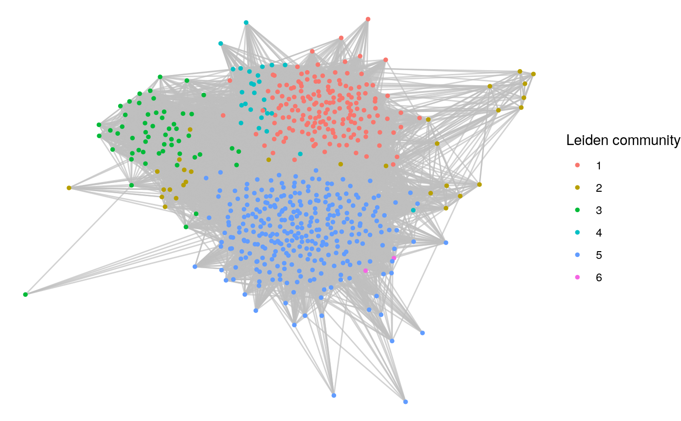
Figure 10.1: Twitter communities of British MPs as detected by the Leiden algorithm
To help characterize each community, we can identify the most important individual in each in terms of degree centrality.
(highest_degree <- tibble(community = 1:max(V(mp_graph_undirected)$cluster)) |>
  dplyr::rowwise() |>
  dplyr::mutate(
    highest_degree = induced_subgraph(
      mp_graph_undirected,
      vids = V(mp_graph_undirected)[V(mp_graph_undirected)$cluster == community]) |>
      degree() |>
      which.max() |>
      names(),
    community_size = V(mp_graph_undirected)[V(mp_graph_undirected)$cluster == community] |>
      length()
  ))
## # A tibble: 6 × 3
## # Rowwise:
## community highest_degree community_size
## <int> <chr> <int>
## 1 1 "Keir Starmer " 163
## 2 2 "Layla Moran" 29
## 3 3 "Philip Davies " 2
## 4 4 "Ian Blackford " 55
## 5 5 "John McDonnell " 35
## 6 6 "Boris Johnson " 301Those with a knowledge of current British politics will be able to identify that the four largest political parties are represented here:
- Boris Johnson at the time of writing is the current Prime Minister and leader of the largest party - The Conservative and Unionist Party
- Sir Keir Starmer is the current leader of the Labour Party
- Ian Blackford is the current parliamentary leader of the Scottish National Party
- Layla Moran is a prominent MP in the Liberal Democratic Party
The other two figures appear to represent clusters which are not well aligned with current party groupings:
- John McDonnell is the former Shadow Chancellor and a member of a leftist faction within the Labour Party. Examination of community 4 will reveal several other members of this leftist faction, such as Jeremy Corbyn and Diane Abbott.
- Philip Davies is a member of the Conservative and Unionist Party, but is currently known as one of the most rebellious MPs in parliament, having voted against his party over 250 times in his career. The other member of this small community of two is his wife Esther McVey, also an MP.
Given that this suggests some alignment of our communities with political party groupings, let’s examine the modularity of the political party communities:
igraph::modularity(
  mp_graph_undirected,
  membership = as.factor(V(mp_graph_undirected)$party)
)
## [1] 0.3560839We can see that the modularity of the political party communities is inferior to our Leiden communities, but the modularities are not dissimilar, suggesting significant overlap. The best way to compare is to visualize the two sets of communities side-by-side, as in Figure 10.2 with the Leiden communities on the left and the ground truth political party communities on the right:
library(patchwork)

# visualize Leiden communities
set.seed(123)
g1 <- ggraph(mp_graph_undirected, layout = "fr") +
  geom_edge_link(color = "grey", alpha = 0.7) +
  geom_node_point(aes(color = factor(cluster)), size = 1, show.legend = FALSE) +
  theme_void()

# visualize ground truth political party communities

party_colours <- mp_vertices |>
  dplyr::select(party, colour) |>
  dplyr::distinct()

set.seed(123)
g2 <- ggraph(mp_graph_undirected, layout = "fr") +
  geom_edge_link(color = "grey", alpha = 0.7) +
  geom_node_point(aes(color = factor(party)), size = 1) +
  theme_void() +
  scale_colour_manual(limits = party_colours$party,
                      values = party_colours$colour, name = "Party (Right Hand Graph)")

# visualize side by side
g1 + g2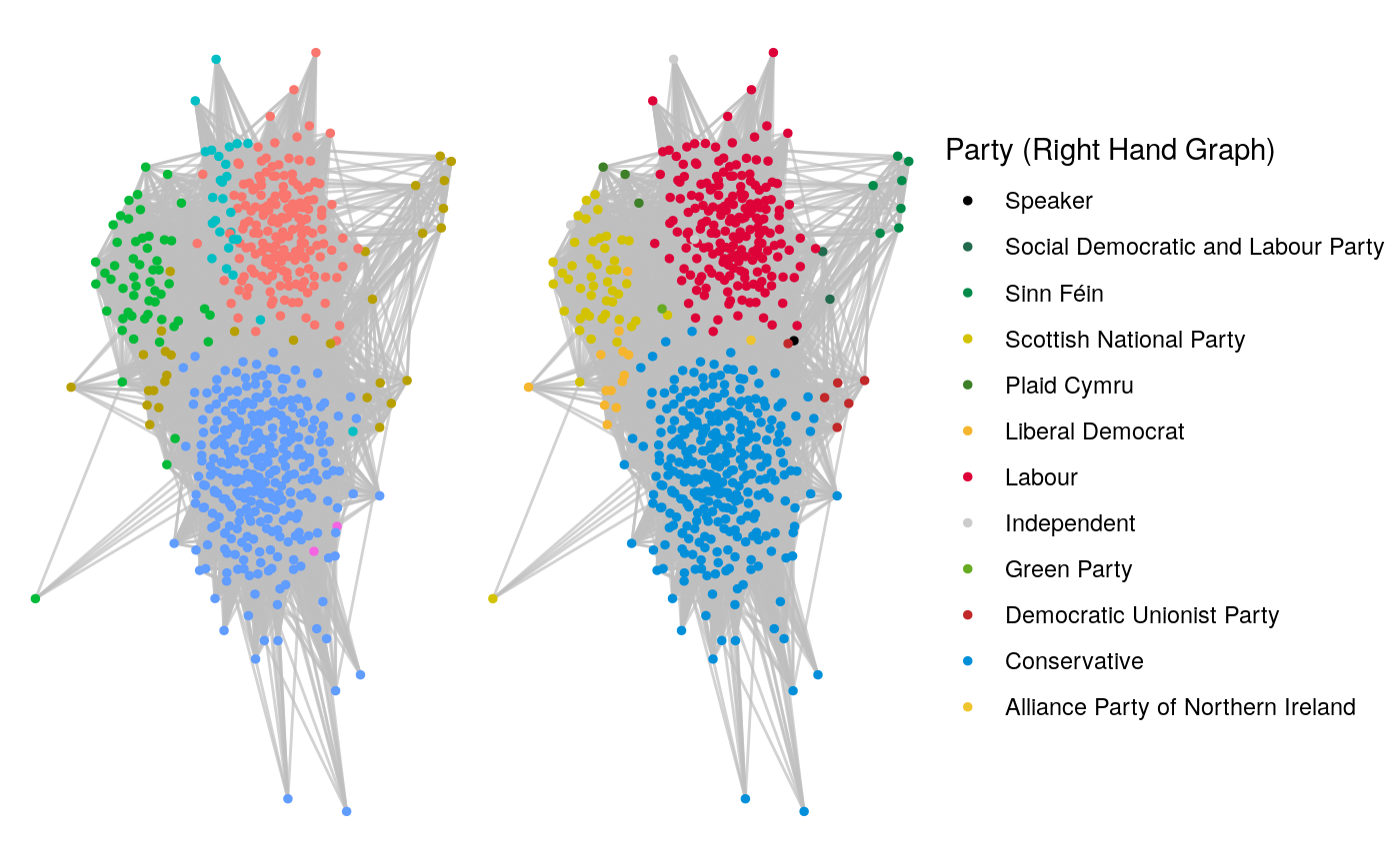
Figure 10.2: Comparison of Leiden communities with ground truth political party communities
It may also be interesting to identify some large cliques in the graph:
(largest_cliques <- igraph::largest_cliques(mp_graph_undirected))## [[1]]
## + 21/585 vertices, named, from cc34729:
## [1] Emily Thornberry Keir Starmer Angela Rayner Boris Johnson Anneliese Dodds
## [6] Yvette Cooper Louise Haigh Lisa Nandy David Lammy Jonathan Ashworth
## [11] Bridget Phillipson Kate Green Sharon Hodgson Nick Thomas-Symonds Edward Miliband
## [16] Jonathan Reynolds Peter Kyle Lucy Powell Vicky Foxcroft Jo Stevens
## [21] Mary Glindon
##
## [[2]]
## + 21/585 vertices, named, from cc34729:
## [1] Emily Thornberry Keir Starmer Angela Rayner Rachel Reeves Anneliese Dodds
## [6] Yvette Cooper David Lammy Louise Haigh Lisa Nandy Jonathan Ashworth
## [11] Bridget Phillipson Sharon Hodgson Lucy Powell Mary Glindon Kate Green
## [16] Jonathan Reynolds Jo Stevens Peter Kyle Nick Thomas-Symonds Edward Miliband
## [21] Vicky Foxcroft
##
## [[3]]
## + 21/585 vertices, named, from cc34729:
## [1] Emily Thornberry Keir Starmer Angela Rayner Rachel Reeves Anneliese Dodds
## [6] Yvette Cooper David Lammy Louise Haigh Lisa Nandy Jonathan Ashworth
## [11] Bridget Phillipson Sharon Hodgson Lucy Powell Tulip Siddiq Peter Kyle
## [16] Kate Green Jo Stevens Jonathan Reynolds Nick Thomas-Symonds Vicky Foxcroft
## [21] Edward Miliband
##
## [[4]]
## + 21/585 vertices, named, from cc34729:
## [1] Emily Thornberry Keir Starmer Angela Rayner Rachel Reeves Anneliese Dodds
## [6] Yvette Cooper David Lammy Louise Haigh Lisa Nandy Jonathan Ashworth
## [11] Bridget Phillipson Sharon Hodgson Lucy Powell Tulip Siddiq Peter Kyle
## [16] Kate Green Gill Furniss Nick Thomas-Symonds Jonathan Reynolds Vicky Foxcroft
## [21] Edward MilibandThese cliques are mostly comprised of members of Labour’s current shadow cabinet. We can also search for the largest Conservative Party clique:
conservative_graph <- igraph::induced_subgraph(
  mp_graph_undirected,
  vids = V(mp_graph_undirected)[V(mp_graph_undirected)$party == "Conservative"]
)

(largest_conservative_cliques <- igraph::largest_cliques(conservative_graph))
## [[1]]
## + 19/308 vertices, named, from 99c3ccb:
## [1] Stephen Barclay Rishi Sunak Boris Johnson Nadhim Zahawi Elizabeth Truss
## [6] Sajid Javid Priti Patel Kwasi Kwarteng Oliver Dowden Nadine Dorries
## [11] Anne-Marie Trevelyan Michael Gove Richard Holden Simon Clarke Michelle Donelan
## [16] Suzanne Webb Brendan Clarke-Smith Eddie Hughes Rachel MacleanThis clique also appears to be mostly consisting of cabinet members. Finally, we can visualize the Labour and Conservative cliques inside the larger graph, as in Figure 10.3, with their central positioning suggesting that these cliques are indeed highly influential, as would be expected given their mostly cabinet membership.
# assign vertices to cliques
V(mp_graph_undirected)$clique <- ifelse(
  V(mp_graph_undirected)$name %in% largest_cliques[[1]]$name,
  "Largest Labour clique",
  ifelse(
    V(mp_graph_undirected)$name %in% largest_conservative_cliques[[1]]$name,
    "Largest Conservative clique",
    "Other"
  )
)

# visualize
set.seed(123)
ggraph(mp_graph_undirected, layout = "fr") +
  geom_edge_link(color = "grey", alpha = 0.7) +
  geom_node_point(aes(color = factor(clique)), size = 1) +
  theme_void() +
  labs(color = "Largest cliques")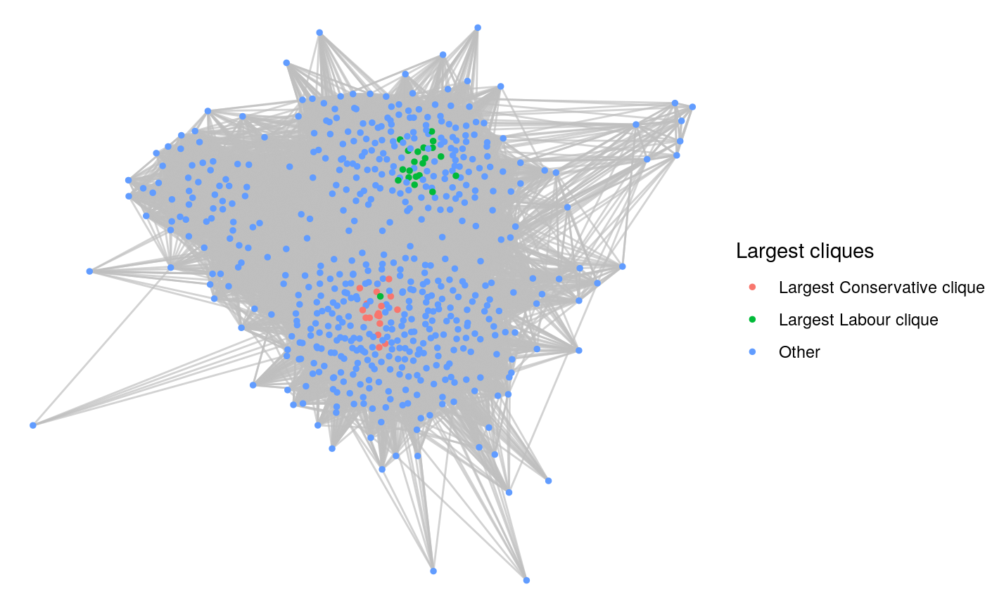
Figure 10.3: Largest Conservative and Labour cliques